Supplemental Figures 12-19
Renee Matthews
2025-02-27
Last updated: 2025-02-27
Checks: 7 0
Knit directory: ATAC_learning/
This reproducible R Markdown analysis was created with workflowr (version 1.7.1). The Checks tab describes the reproducibility checks that were applied when the results were created. The Past versions tab lists the development history.
Great! Since the R Markdown file has been committed to the Git repository, you know the exact version of the code that produced these results.
Great job! The global environment was empty. Objects defined in the global environment can affect the analysis in your R Markdown file in unknown ways. For reproduciblity it’s best to always run the code in an empty environment.
The command set.seed(20231016) was run prior to running
the code in the R Markdown file. Setting a seed ensures that any results
that rely on randomness, e.g. subsampling or permutations, are
reproducible.
Great job! Recording the operating system, R version, and package versions is critical for reproducibility.
Nice! There were no cached chunks for this analysis, so you can be confident that you successfully produced the results during this run.
Great job! Using relative paths to the files within your workflowr project makes it easier to run your code on other machines.
Great! You are using Git for version control. Tracking code development and connecting the code version to the results is critical for reproducibility.
The results in this page were generated with repository version 8435f1f. See the Past versions tab to see a history of the changes made to the R Markdown and HTML files.
Note that you need to be careful to ensure that all relevant files for
the analysis have been committed to Git prior to generating the results
(you can use wflow_publish or
wflow_git_commit). workflowr only checks the R Markdown
file, but you know if there are other scripts or data files that it
depends on. Below is the status of the Git repository when the results
were generated:
Ignored files:
    Ignored:    .RData
    Ignored:    .Rhistory
    Ignored:    .Rproj.user/
    Ignored:    analysis/figure/
    Ignored:    data/ACresp_SNP_table.csv
    Ignored:    data/ARR_SNP_table.csv
    Ignored:    data/All_merged_peaks.tsv
    Ignored:    data/CAD_gwas_dataframe.RDS
    Ignored:    data/CTX_SNP_table.csv
    Ignored:    data/Collapsed_expressed_NG_peak_table.csv
    Ignored:    data/DEG_toplist_sep_n45.RDS
    Ignored:    data/FRiP_first_run.txt
    Ignored:    data/Final_four_data/
    Ignored:    data/Frip_1_reads.csv
    Ignored:    data/Frip_2_reads.csv
    Ignored:    data/Frip_3_reads.csv
    Ignored:    data/Frip_4_reads.csv
    Ignored:    data/Frip_5_reads.csv
    Ignored:    data/Frip_6_reads.csv
    Ignored:    data/GO_KEGG_analysis/
    Ignored:    data/HF_SNP_table.csv
    Ignored:    data/Ind1_75DA24h_dedup_peaks.csv
    Ignored:    data/Ind1_TSS_peaks.RDS
    Ignored:    data/Ind1_firstfragment_files.txt
    Ignored:    data/Ind1_fragment_files.txt
    Ignored:    data/Ind1_peaks_list.RDS
    Ignored:    data/Ind1_summary.txt
    Ignored:    data/Ind2_TSS_peaks.RDS
    Ignored:    data/Ind2_fragment_files.txt
    Ignored:    data/Ind2_peaks_list.RDS
    Ignored:    data/Ind2_summary.txt
    Ignored:    data/Ind3_TSS_peaks.RDS
    Ignored:    data/Ind3_fragment_files.txt
    Ignored:    data/Ind3_peaks_list.RDS
    Ignored:    data/Ind3_summary.txt
    Ignored:    data/Ind4_79B24h_dedup_peaks.csv
    Ignored:    data/Ind4_TSS_peaks.RDS
    Ignored:    data/Ind4_V24h_fraglength.txt
    Ignored:    data/Ind4_fragment_files.txt
    Ignored:    data/Ind4_fragment_filesN.txt
    Ignored:    data/Ind4_peaks_list.RDS
    Ignored:    data/Ind4_summary.txt
    Ignored:    data/Ind5_TSS_peaks.RDS
    Ignored:    data/Ind5_fragment_files.txt
    Ignored:    data/Ind5_fragment_filesN.txt
    Ignored:    data/Ind5_peaks_list.RDS
    Ignored:    data/Ind5_summary.txt
    Ignored:    data/Ind6_TSS_peaks.RDS
    Ignored:    data/Ind6_fragment_files.txt
    Ignored:    data/Ind6_peaks_list.RDS
    Ignored:    data/Ind6_summary.txt
    Ignored:    data/Knowles_4.RDS
    Ignored:    data/Knowles_5.RDS
    Ignored:    data/Knowles_6.RDS
    Ignored:    data/LiSiLTDNRe_TE_df.RDS
    Ignored:    data/MI_gwas.RDS
    Ignored:    data/SNP_GWAS_PEAK_MRC_id
    Ignored:    data/SNP_GWAS_PEAK_MRC_id.csv
    Ignored:    data/SNP_gene_cat_list.tsv
    Ignored:    data/SNP_supp_schneider.RDS
    Ignored:    data/TE_info/
    Ignored:    data/TFmapnames.RDS
    Ignored:    data/all_TSSE_scores.RDS
    Ignored:    data/all_four_filtered_counts.txt
    Ignored:    data/aln_run1_results.txt
    Ignored:    data/anno_ind1_DA24h.RDS
    Ignored:    data/anno_ind4_V24h.RDS
    Ignored:    data/annotated_gwas_SNPS.csv
    Ignored:    data/background_n45_he_peaks.RDS
    Ignored:    data/cardiac_muscle_FRIP.csv
    Ignored:    data/cardiomyocyte_FRIP.csv
    Ignored:    data/col_ng_peak.csv
    Ignored:    data/cormotif_full_4_run.RDS
    Ignored:    data/cormotif_full_4_run_he.RDS
    Ignored:    data/cormotif_full_6_run.RDS
    Ignored:    data/cormotif_full_6_run_he.RDS
    Ignored:    data/cormotif_probability_45_list.csv
    Ignored:    data/cormotif_probability_45_list_he.csv
    Ignored:    data/cormotif_probability_all_6_list.csv
    Ignored:    data/cormotif_probability_all_6_list_he.csv
    Ignored:    data/datasave.RDS
    Ignored:    data/embryo_heart_FRIP.csv
    Ignored:    data/enhancer_list_ENCFF126UHK.bed
    Ignored:    data/enhancerdata/
    Ignored:    data/filt_Peaks_efit2.RDS
    Ignored:    data/filt_Peaks_efit2_bl.RDS
    Ignored:    data/filt_Peaks_efit2_n45.RDS
    Ignored:    data/first_Peaksummarycounts.csv
    Ignored:    data/first_run_frag_counts.txt
    Ignored:    data/full_bedfiles/
    Ignored:    data/gene_ref.csv
    Ignored:    data/gwas_1_dataframe.RDS
    Ignored:    data/gwas_2_dataframe.RDS
    Ignored:    data/gwas_3_dataframe.RDS
    Ignored:    data/gwas_4_dataframe.RDS
    Ignored:    data/gwas_5_dataframe.RDS
    Ignored:    data/high_conf_peak_counts.csv
    Ignored:    data/high_conf_peak_counts.txt
    Ignored:    data/high_conf_peaks_bl_counts.txt
    Ignored:    data/high_conf_peaks_counts.txt
    Ignored:    data/hits_files/
    Ignored:    data/hyper_files/
    Ignored:    data/hypo_files/
    Ignored:    data/ind1_DA24hpeaks.RDS
    Ignored:    data/ind1_TSSE.RDS
    Ignored:    data/ind2_TSSE.RDS
    Ignored:    data/ind3_TSSE.RDS
    Ignored:    data/ind4_TSSE.RDS
    Ignored:    data/ind4_V24hpeaks.RDS
    Ignored:    data/ind5_TSSE.RDS
    Ignored:    data/ind6_TSSE.RDS
    Ignored:    data/initial_complete_stats_run1.txt
    Ignored:    data/left_ventricle_FRIP.csv
    Ignored:    data/median_24_lfc.RDS
    Ignored:    data/median_3_lfc.RDS
    Ignored:    data/mergedPeads.gff
    Ignored:    data/mergedPeaks.gff
    Ignored:    data/motif_list_full
    Ignored:    data/motif_list_n45
    Ignored:    data/motif_list_n45.RDS
    Ignored:    data/multiqc_fastqc_run1.txt
    Ignored:    data/multiqc_fastqc_run2.txt
    Ignored:    data/multiqc_genestat_run1.txt
    Ignored:    data/multiqc_genestat_run2.txt
    Ignored:    data/my_hc_filt_counts.RDS
    Ignored:    data/my_hc_filt_counts_n45.RDS
    Ignored:    data/n45_bedfiles/
    Ignored:    data/n45_files
    Ignored:    data/other_papers/
    Ignored:    data/peakAnnoList_1.RDS
    Ignored:    data/peakAnnoList_2.RDS
    Ignored:    data/peakAnnoList_24_full.RDS
    Ignored:    data/peakAnnoList_24_n45.RDS
    Ignored:    data/peakAnnoList_3.RDS
    Ignored:    data/peakAnnoList_3_full.RDS
    Ignored:    data/peakAnnoList_3_n45.RDS
    Ignored:    data/peakAnnoList_4.RDS
    Ignored:    data/peakAnnoList_5.RDS
    Ignored:    data/peakAnnoList_6.RDS
    Ignored:    data/peakAnnoList_Eight.RDS
    Ignored:    data/peakAnnoList_full_motif.RDS
    Ignored:    data/peakAnnoList_n45_motif.RDS
    Ignored:    data/siglist_full.RDS
    Ignored:    data/siglist_n45.RDS
    Ignored:    data/summarized_peaks_dataframe.txt
    Ignored:    data/summary_peakIDandReHeat.csv
    Ignored:    data/test.list.RDS
    Ignored:    data/testnames.txt
    Ignored:    data/toplist_6.RDS
    Ignored:    data/toplist_full.RDS
    Ignored:    data/toplist_full_DAR_6.RDS
    Ignored:    data/toplist_n45.RDS
    Ignored:    data/trimmed_seq_length.csv
    Ignored:    data/unclassified_full_set_peaks.RDS
    Ignored:    data/unclassified_n45_set_peaks.RDS
    Ignored:    data/xstreme/

Untracked files:
    Untracked:  analysis/Expressed_RNA_associations.Rmd
    Untracked:  analysis/LFC_corr.Rmd
    Untracked:  analysis/SVA.Rmd
    Untracked:  analysis/Tan2020.Rmd
    Untracked:  analysis/my_hc_filt_counts.csv
    Untracked:  code/IGV_snapshot_code.R
    Untracked:  code/LongDARlist.R
    Untracked:  code/just_for_Fun.R
    Untracked:  output/cormotif_probability_45_list.csv
    Untracked:  output/cormotif_probability_all_6_list.csv
    Untracked:  setup.RData

Unstaged changes:
    Modified:   ATAC_learning.Rproj
    Modified:   analysis/Correlation_of_SNPnPEAK.Rmd
    Modified:   analysis/Figure_1.Rmd
    Modified:   analysis/GO_KEGG_analysis.Rmd
    Modified:   analysis/Raodah_mycount.Rmd
    Modified:   analysis/TE_analysis_ff.Rmd
    Modified:   analysis/final_four_analysis.Rmd
    Modified:   analysis/final_plot_attempt.Rmd
    Modified:   analysis/index.Rmd
Note that any generated files, e.g. HTML, png, CSS, etc., are not included in this status report because it is ok for generated content to have uncommitted changes.
These are the previous versions of the repository in which changes were
made to the R Markdown (analysis/Supp_Fig_12-19.Rmd) and
HTML (docs/Supp_Fig_12-19.html) files. If you’ve configured
a remote Git repository (see ?wflow_git_remote), click on
the hyperlinks in the table below to view the files as they were in that
past version.
| File | Version | Author | Date | Message |
|---|---|---|---|---|
| Rmd | 8435f1f | E. Renee Matthews | 2025-02-27 | adding figures |
| Rmd | fcc1425 | E. Renee Matthews | 2025-02-27 | Build site. |
| Rmd | 337980a | E. Renee Matthews | 2025-02-27 | updates to plot |
| Rmd | 37c7d47 | E. Renee Matthews | 2025-02-27 | wflow_git_commit("analysis/Supp_Fig_12-19.Rmd") |
library(tidyverse)
library(kableExtra)
library(broom)
library(RColorBrewer)
library(ChIPseeker)
library("TxDb.Hsapiens.UCSC.hg38.knownGene")
library("org.Hs.eg.db")
library(rtracklayer)
library(ggfortify)
library(readr)
library(BiocGenerics)
library(gridExtra)
library(VennDiagram)
library(scales)
library(ggVennDiagram)
library(BiocParallel)
library(ggpubr)
library(edgeR)
library(genomation)
library(ggsignif)
library(plyranges)
library(ggrepel)
library(ComplexHeatmap)
library(cowplot)
library(smplot2)
library(readxl)
library(devtools)
library(vargen)
library(eulerr)
Figure S12: H3K27ac Enrichment at TSS
knitr::include_graphics("assets/Fig\ S12.png", error=FALSE)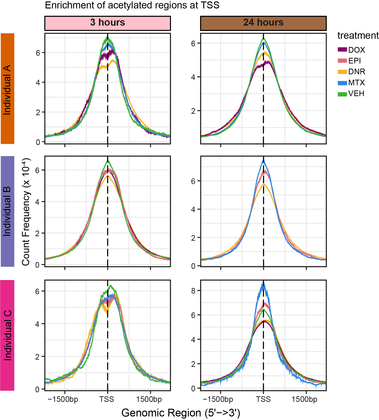
| Version | Author | Date |
|---|---|---|
| 50f3de9 | E. Renee Matthews | 2025-02-21 |
knitr::include_graphics("docs/assets/Fig\ S12.png",error = FALSE)
txdb <- TxDb.Hsapiens.UCSC.hg38.knownGene
###taken from Peak_calling rmd

# first get peakfiles (using .narrowPeak files from MACS2 calling) and upload functions

TSS = getBioRegion(TxDb=txdb, upstream=2000, downstream=2000, by = "gene",
                   type = "start_site")
#### EXAMPLE OF CODE #####
# ind4_V24hpeaks_gr <- prepGRangeObj(ind4_V24hpeaks)
# ind1_DA24hpeaks_gr <- prepGRangeObj((ind1_DA24hpeaks))
# H3K27ac_list <- GRangesList(ind1_DA24hpeaks_gr, ind4_V24hpeaks_gr)
# # ##plotting the TSS average window (making an overlap of each using Epi_list as list holder)
# H3K27ac_list_tagMatrix = lapply(H3K27ac_list, getTagMatrix, windows = TSS)
# plotAvgProf(H3K27ac_list_tagMatrix, xlim=c(-3000, 3000), ylab = "Count Frequency")
#plotPeakProf(H3K27ac_list_tagMatrix, facet = "none", conf = 0.95)

## What I did here:  I called all my narrowpeak files
peakfiles1 <- choose.files()

##these were practice for getting file names and shortening for the for loop below
# testname <- basename(peakfiles1[1])
# str_split_i(testname, "_",3)

##This loop first established a list then (because I already knew the list had 12 files)
## I then imported each of these onto that list.  Once I had the list, I stored it as
## an R object,
IndA_peaks <- list()
for (file in 1:8){
    testname <- basename(peakfiles1[file])
  banana_peel <- str_split_i(testname, "_",3)
 IndA_peaks[[banana_peel]] <- readPeakFile(peakfiles1[file])
}
saveRDS(IndA_peaks, "data/Final_four_data/H3K27ac_files/IndA_peaks_list.RDS")
# I then called annotatePeak on that list object, and stored that as a R object for later retrieval.)
peakAnnoList_1 <- lapply(IndA_peaks, annotatePeak, tssRegion =c(-2000,2000), TxDb= txdb)
saveRDS(peakAnnoList_1, "data/Final_four_data/H3K27ac_files/IndA_peakAnnoList.RDS")
promoter <- getPromoters(TxDb=txdb, upstream=3000, downstream=3000)
tagMatrix_C <- lapply(IndC_peaks,getTagMatrix, windows=promoter)
plotAvgProf(tagMatrix_C, xlim = c(-3000,3000),xlab = "Genomic Region (5'->3')", ylab = "Read Count Frequency")

saveRDS(tagMatrix_C, "data/Final_four_data/H3K27ac_files/IndC_tagMatrix.RDS")
Making the plot
##load tagMatrix files from above
tagMatrix_A <- readRDS("data/Final_four_data/H3K27ac_files/IndA_tagMatrix.RDS")
tagMatrix_B <- readRDS("data/Final_four_data/H3K27ac_files/IndB_tagMatrix.RDS")
tagMatrix_C <- readRDS("data/Final_four_data/H3K27ac_files/IndC_tagMatrix.RDS")
###making the plots and storing the 3 hour as an object
a1<- plotAvgProf(tagMatrix_A[c(1,3,5,7)], xlim=c(-3000, 3000), ylab = "Count Frequency")+ ggtitle("3 hour Individual A" )+coord_cartesian(xlim=c(-2000,2000))
>> plotting figure... 2025-02-27 5:56:37 PM b1 <- plotAvgProf(tagMatrix_B[c(1,3,4,7)], xlim=c(-3000, 3000), ylab = "Count Frequency")+ ggtitle("3 hour Individual B" )+coord_cartesian(xlim=c(-2000,2000))>> plotting figure... 2025-02-27 5:56:37 PM c1 <- plotAvgProf(tagMatrix_C[c(1,4,6,8)], xlim=c(-3000, 3000), ylab = "Count Frequency")+ ggtitle("3 hour Individual C" )+coord_cartesian(xlim=c(-2000,2000))>> plotting figure... 2025-02-27 5:56:38 PM ### making the plots and storing the 24 hour as an object
a2<- plotAvgProf(tagMatrix_A[c(2,4,6,8)], xlim=c(-3000, 3000), ylab = "Count Frequency")+ ggtitle("24 hour Individual A" )+coord_cartesian(xlim=c(-2000,2000))>> plotting figure... 2025-02-27 5:56:38 PM b2 <- plotAvgProf(tagMatrix_B[c(2,5,6,8)], xlim=c(-3000, 3000), ylab = "Count Frequency")+ ggtitle("24 hour Individual B" )+coord_cartesian(xlim=c(-2000,2000))>> plotting figure... 2025-02-27 5:56:38 PM c2 <- plotAvgProf(tagMatrix_C[c(2,3,5,7,9)], xlim=c(-3000, 3000), ylab = "Count Frequency")+ ggtitle("24 hour Individual C" )+coord_cartesian(xlim=c(-2000,2000))>> plotting figure... 2025-02-27 5:56:38 PM plot_grid(a1,a2, b1,b2,c1,c2, axis="l",align = "hv",nrow=3, ncol=2)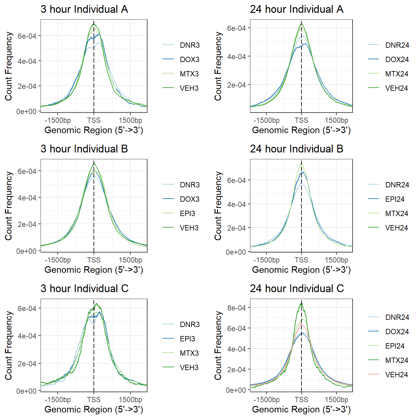
Figure S13: Correlation between H3K27ac enrichment across samples
H3K27ac_counts <- read_delim("data/Final_four_data/H3K27ac_files/H3K27ac_counts_file.txt", delim= "\t")
corr_lcpmH3K27ac <- H3K27ac_counts %>%
  column_to_rownames("Geneid") %>%
  cpm(.,log=TRUE) %>%
  cor()

filmat_groupmat_col <- data.frame(timeset = colnames(corr_lcpmH3K27ac))

counts_corr_mat <-  filmat_groupmat_col %>%
  separate(timeset, into = c("indv","trt","time"), sep= "_") %>%
  mutate(time = factor(time, levels = c("3", "24"), labels= c("3 hours","24 hours"))) %>%
  mutate(trt = factor(trt, levels = c("DOX","EPI", "DNR", "MTX","VEH"))) %>%
  mutate(class = if_else(trt == "DNR", "AC", if_else(
    trt == "DOX", "AC", if_else(trt == "EPI", "AC", "nAC")
  ))) %>%
  mutate(TOP2i = if_else(trt == "DNR", "yes", if_else(
    trt == "DOX", "yes", if_else(trt == "EPI", "yes", if_else(trt == "MTX", "yes", "no"))))) %>%
  mutate(indv=factor(indv, levels = c("A","B","C")))

 mat_colors <- list(
   trt= c("#F1B72B","#8B006D","#DF707E","#3386DD","#41B333"),
   indv=c(A="#1B9E77",B= "#D95F02" ,C="#7570B3"),
   time=c("pink", "chocolate4"),
   class=c("yellow1","darkorange1"),
   TOP2i =c("darkgreen","lightgreen"))

names(mat_colors$trt)   <- unique(counts_corr_mat$trt)
names(mat_colors$indv) <- unique(counts_corr_mat$indv)
names(mat_colors$time) <- unique(counts_corr_mat$time)
names(mat_colors$class) <- unique(counts_corr_mat$class)
names(mat_colors$TOP2i) <- unique(counts_corr_mat$TOP2i)

htanno <-  ComplexHeatmap::HeatmapAnnotation(df = counts_corr_mat, col = mat_colors)
ComplexHeatmap::Heatmap(corr_lcpmH3K27ac, top_annotation = htanno)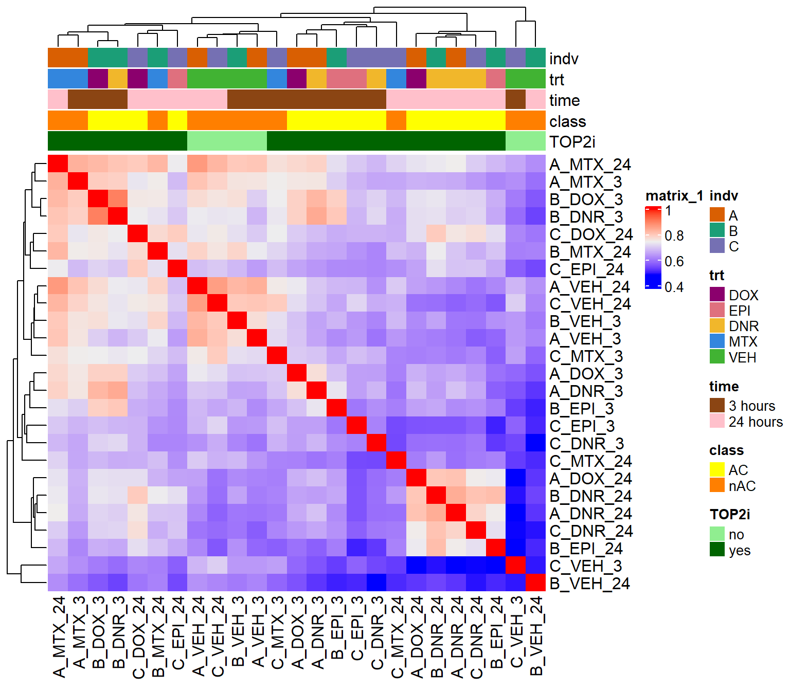
Figure S14: H3K27-acetylation response is highly correlated across ACs
Figure S14A: Differentially enriched H3K27ac regions across drug treatments
Code for Differential analysis
### group  without veh3hr and veh24hr individual samples
# group_23s <- c( 1,2,4,5,6,7,10,1,2,3,4,7,8,9,10,1,2,3,5,6,7,8,9)
H3K27ac_counts_file <- read_delim("data/Final_four_data/H3K27ac_files/H3K27ac_counts_file.txt", delim= "\t")
PCA_H3_mat_23s <- H3K27ac_counts_file %>%
  ##removing C_VEH_3 and B_VEH_24 columns
  dplyr::select(Geneid,B_DNR_24:B_MTX_24, B_VEH_3:C_VEH_24) %>%
  column_to_rownames("Geneid") %>%
  as.matrix()

anno_H3_mat_23s <-
data.frame(timeset=colnames(PCA_H3_mat_23s)) %>%
  mutate(sample = timeset) %>%
  separate(timeset, into = c("indv","trt","time"), sep= "_") %>%
  mutate(time = factor(time, levels = c("3", "24"), labels= c("3 hours","24 hours"))) %>%
  mutate(trt = factor(trt, levels = c("DOX","EPI", "DNR", "MTX","VEH")))


lcpm_h3_23s <- cpm(PCA_H3_mat_23s, log=TRUE)  ### for determining the basic cutoffs
row_means23s <- rowMeans(lcpm_h3_23s)
h3_23s_filtered <- PCA_H3_mat_23s[row_means23s >0,]
filt_H3_matrix_lcpm_23s <- cpm(h3_23s_filtered, log=TRUE)

### no difference in between filtered and unfiltered numbers

for_group_23s <- data.frame(timeset=colnames(PCA_H3_mat_23s)) %>%
  mutate(sample = timeset) %>%
  separate(timeset, into = c("indv","trt","time"), sep= "_") %>%
  unite("test", trt:time,sep="_", remove = FALSE)

# dge_23s <- DGEList.data.frame(counts = PCA_H3_mat_23s, group = group_23s, genes = lcpm_h3_23s_filtered)

# group_1 <- for_group_23s$test
#
# dge_23s$group$indv <- for_group_23s$indv
# dge_23s$group$time <- for_group_23s$time
# dge_23s$group$trt <- for_group_23s$trt
# #
# indv_23s <- for_group_23s$indv
# mm <- model.matrix(~0 +group_1)
# colnames(mm) <-  c("DNR_24", "DNR_3", "DOX_24","DOX_3","EPI_24", "EPI_3","MTX_24", "MTX_3","VEH_24", "VEH_3")
#
# y <- voom(dge_23s$counts, mm,plot =TRUE)
#
# corfit <- duplicateCorrelation(y, mm, block = indv_23s)
#
# v <- voom(dge_23s$counts, mm, block = indv_23s, correlation = corfit$consensus)
#
# fit <- lmFit(v, mm, block = indv_23s, correlation = corfit$consensus)
# # colnames(mm) <- c("DNR_24","DNR_3","DOX_24","DOX_3","EPI_24","EPI_3","MTX_24","MTX_3","TRZ_24","TRZ_3","VEH_24", "VEH_3")
# #
# #
# cm <- makeContrasts(
#   DNR_3.VEH_3 = DNR_3-VEH_3,
#   DOX_3.VEH_3 = DOX_3-VEH_3,
#   EPI_3.VEH_3 = EPI_3-VEH_3,
#   MTX_3.VEH_3 = MTX_3-VEH_3,
#   DNR_24.VEH_24 =DNR_24-VEH_24,
#   DOX_24.VEH_24= DOX_24-VEH_24,
#   EPI_24.VEH_24= EPI_24-VEH_24,
#   MTX_24.VEH_24= MTX_24-VEH_24,
#     levels = mm)
#
# vfit <- lmFit(y, mm)
# #
# vfit<- contrasts.fit(vfit, contrasts=cm)
#
# efit4_raodah_23s <- eBayes(vfit)
efit_raodah_23s <- readRDS("data/Final_four_data/efit4_raodah_23s.RDS")
results = decideTests(efit_raodah_23s)
summary(results) DNR_3.VEH_3 DOX_3.VEH_3 EPI_3.VEH_3 MTX_3.VEH_3 DNR_24.VEH_24
Down 424 2 0 0 2007
NotSig 19502 20135 20137 20137 16669
Up 211 0 0 0 1461
DOX_24.VEH_24 EPI_24.VEH_24 MTX_24.VEH_24
Down 126 55 0
NotSig 19756 19997 20137
Up 255 85 0AC.DNR_3.top= topTable(efit_raodah_23s, coef=1, adjust.method="BH", number=Inf, sort.by="p")
AC.DOX_3.top= topTable(efit_raodah_23s, coef=2, adjust.method="BH", number=Inf, sort.by="p")
AC.EPI_3.top= topTable(efit_raodah_23s, coef=3, adjust.method="BH", number=Inf, sort.by="p")
AC.MTX_3.top= topTable(efit_raodah_23s, coef=4, adjust.method="BH", number=Inf, sort.by="p")
AC.DNR_24.top= topTable(efit_raodah_23s, coef=5, adjust.method="BH", number=Inf, sort.by="p")
AC.DOX_24.top= topTable(efit_raodah_23s, coef=6, adjust.method="BH", number=Inf, sort.by="p")
AC.EPI_24.top= topTable(efit_raodah_23s, coef=7, adjust.method="BH", number=Inf, sort.by="p")
AC.MTX_24.top= topTable(efit_raodah_23s, coef=8, adjust.method="BH", number=Inf, sort.by="p")
plot_filenames <- c("AC.DNR_3.top","AC.DOX_3.top","AC.EPI_3.top","AC.MTX_3.top",
"AC.DNR_24.top","AC.DOX_24.top","AC.EPI_24.top",
"AC.MTX_24.top")
plot_files <- c( AC.DNR_3.top,AC.DOX_3.top,AC.EPI_3.top,AC.MTX_3.top,
AC.DNR_24.top,AC.DOX_24.top,AC.EPI_24.top,
AC.MTX_24.top)
volcanosig <- function(df, psig.lvl) {
df <- df %>%
mutate(threshold = ifelse(adj.P.Val > psig.lvl, "A", ifelse(adj.P.Val <= psig.lvl & logFC<=0,"B","C")))
ggplot(df, aes(x=logFC, y=-log10(P.Value))) +
geom_point(aes(color=threshold))+
xlab(expression("Log"[2]*" FC"))+
ylab(expression("-log"[10]*"P Value"))+
scale_color_manual(values = c("black", "red","blue"))+
ylim(0,12)+
xlim(-5,5)+
theme_cowplot()+
theme(legend.position = "none",
plot.title = element_text(size = rel(1.5), hjust = 0.5),
axis.title = element_text(size = rel(0.8)))
}
v1 <- volcanosig(AC.DNR_3.top, 0.05)+ ggtitle("H3K27ac DNR 3 hour")
v2 <- volcanosig(AC.DNR_24.top, 0.05)+ ggtitle("H3K27ac DNR 24 hour")+ylab("")
v3 <- volcanosig(AC.DOX_3.top, 0.05)+ ggtitle("H3K27ac DOX 3 hour")
v4 <- volcanosig(AC.DOX_24.top, 0.05)+ ggtitle("H3K27ac DOX 24 hour")+ylab("")
v5 <- volcanosig(AC.EPI_3.top, 0.05)+ ggtitle("H3K27ac EPI 3 hour")
v6 <- volcanosig(AC.EPI_24.top, 0.05)+ ggtitle("H3K27ac EPI 24 hour")+ylab("")
v7 <- volcanosig(AC.MTX_3.top, 0.05)+ ggtitle("H3K27ac MTX 3 hour")
v8 <- volcanosig(AC.MTX_24.top, 0.05)+ ggtitle("H3K27ac MTX 24 hour")+ylab("")
plot_grid(v1,v2, rel_widths =c(.8,1))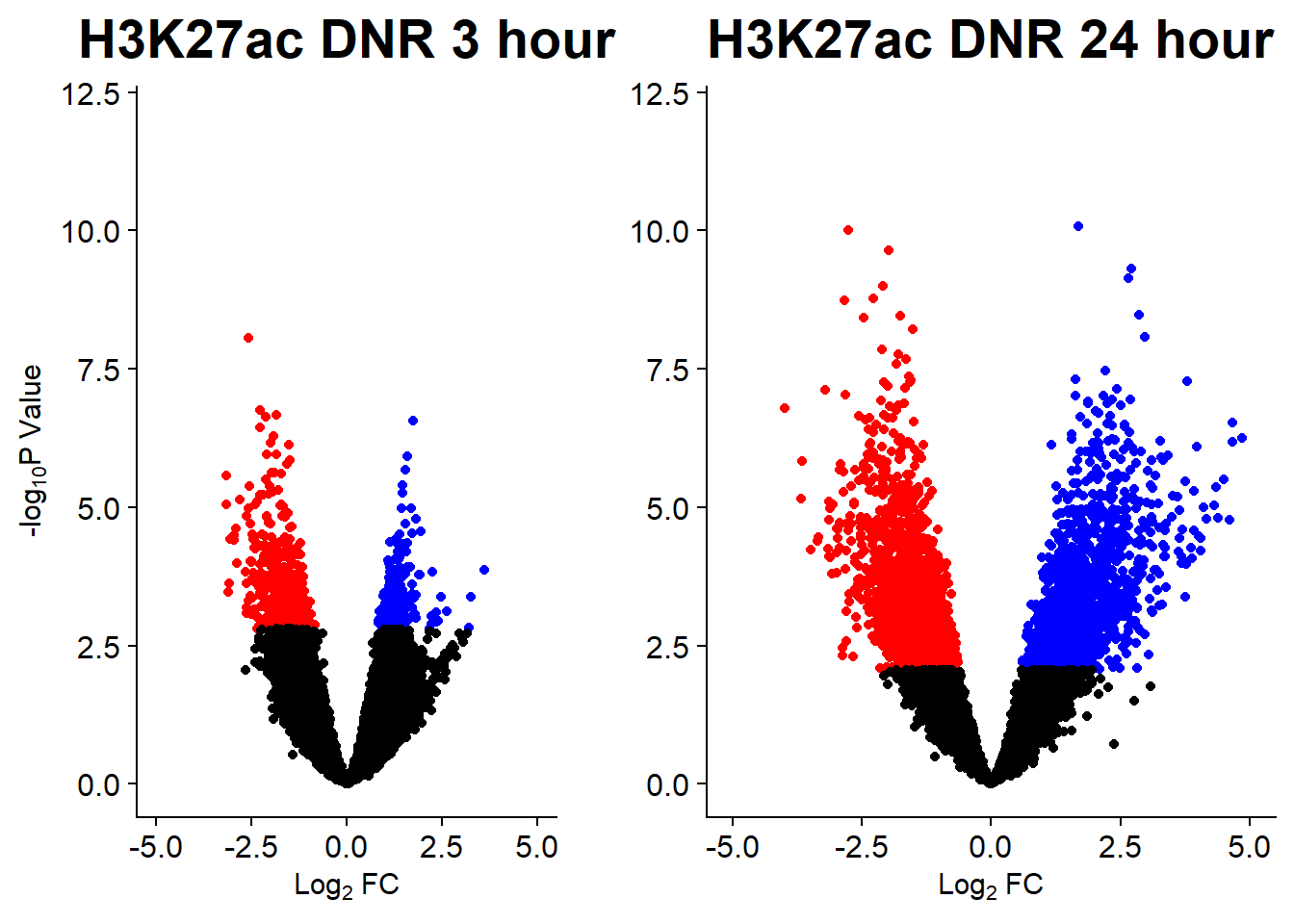
plot_grid(v3,v4, rel_widths =c(.8,1))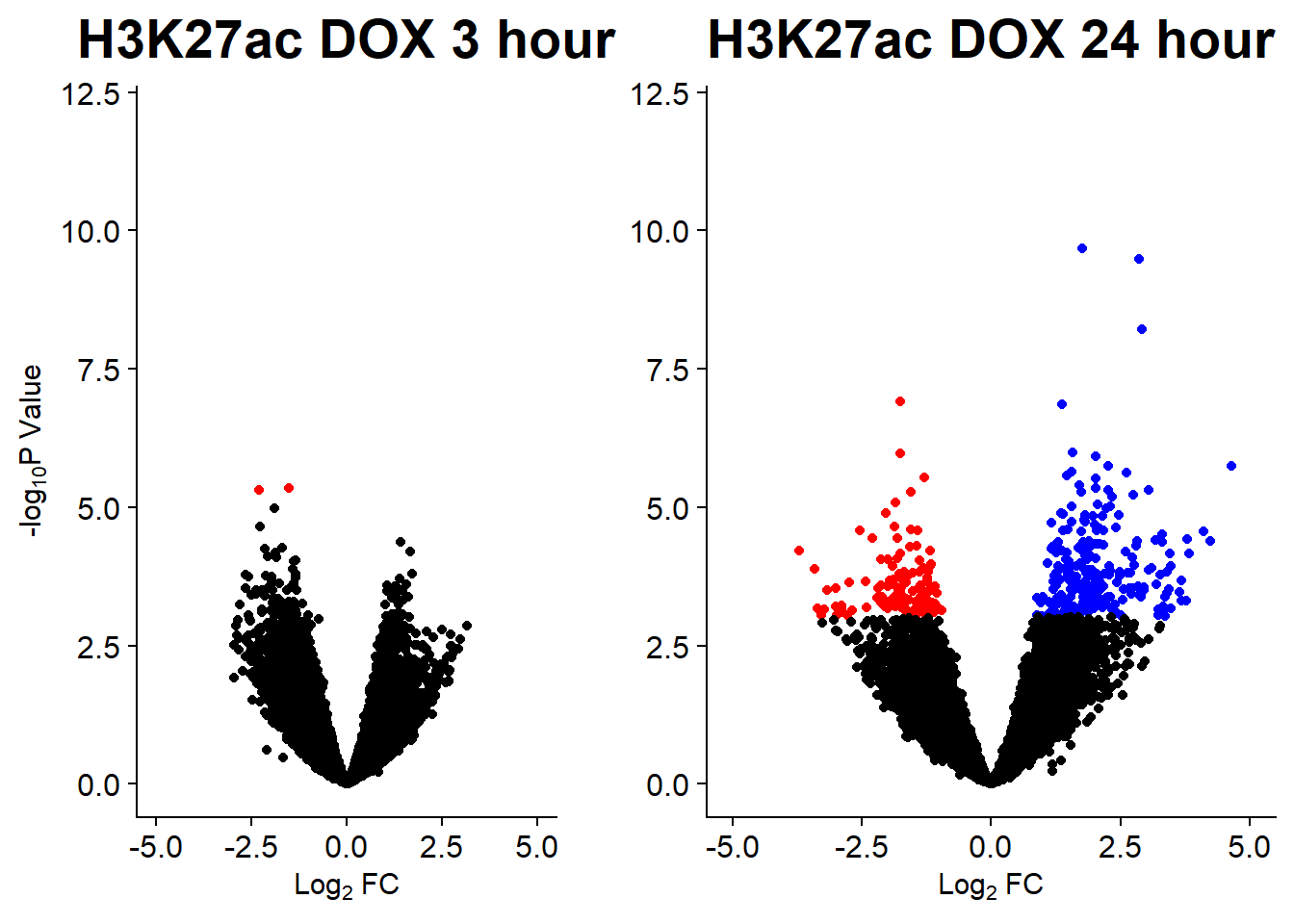
plot_grid(v5,v6, rel_widths =c(.8,1))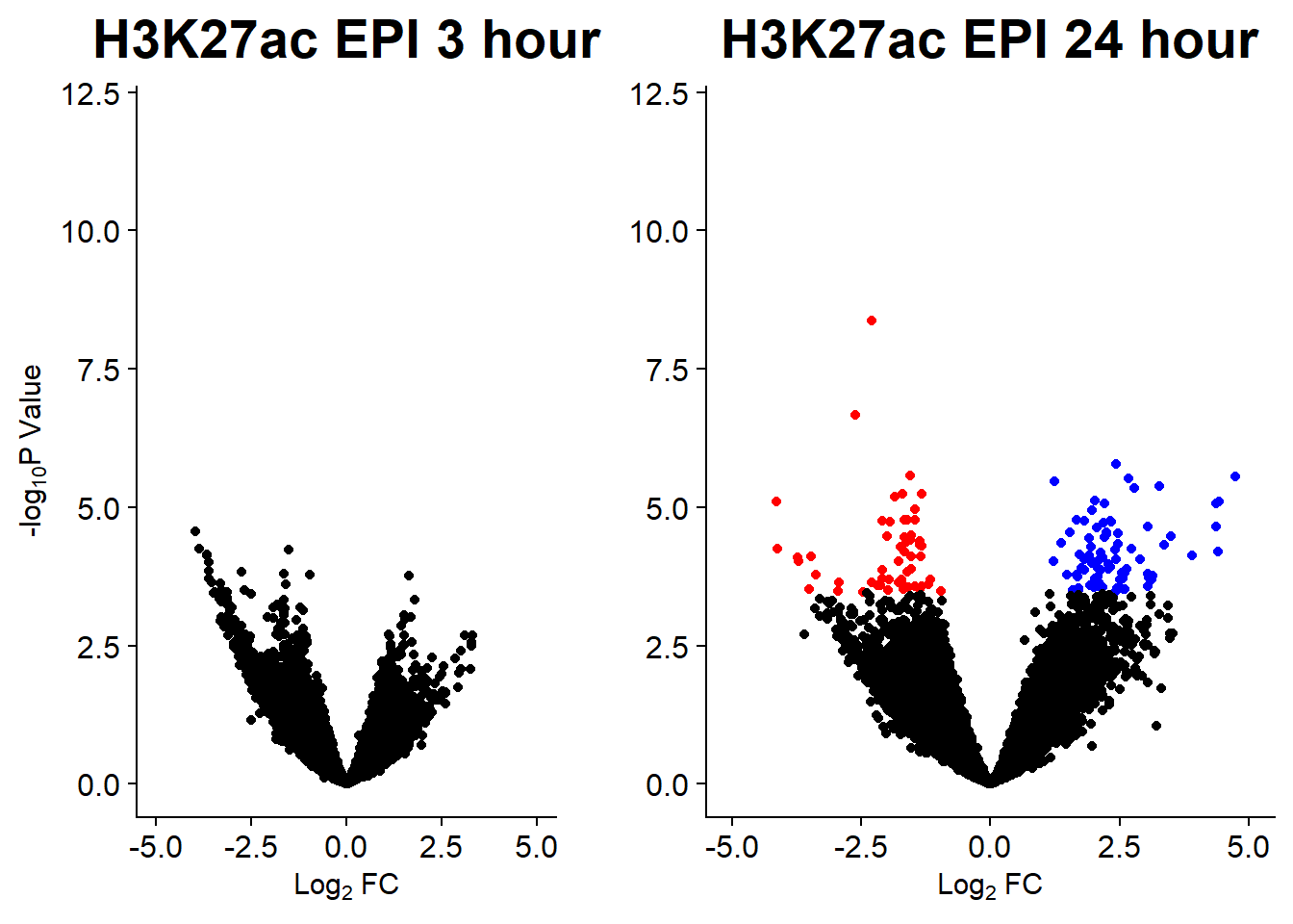
plot_grid(v7,v8, rel_widths =c(.8,1))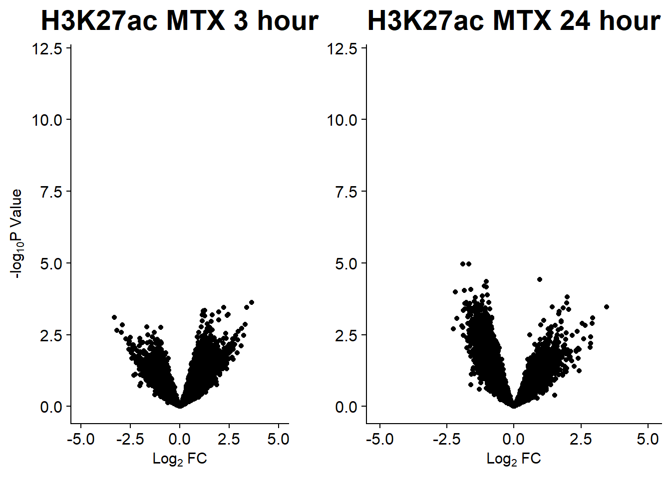 #### Figure S14B:
FCmatrix_23s <- subset(efit_raodah_23s$coefficients)

colnames(FCmatrix_23s) <-
  c("DNR\n3h",
    "DOX\n3h",
    "EPI\n3h",
    "MTX\n3h",
    "DNR\n24h",
    "DOX\n24h",
    "EPI\n24h",
    "MTX\n24h"
     )


mat_col_FC <-
  data.frame(
    time = c(rep("3 hours", 4), rep("24 hours", 4)),
    class = (c(
      "AC", "AC", "AC", "nAC", "AC", "AC", "AC", "nAC"
    )))
rownames(mat_col_FC) <- colnames(FCmatrix_23s)

mat_colors_FC <-
  list(
    time = c("pink", "chocolate4"),
    class = c("yellow1", "lightgreen"))

names(mat_colors_FC$time) <- unique(mat_col_FC$time)
names(mat_colors_FC$class) <- unique(mat_col_FC$class)
# names(mat_colors_FC$TOP2i) <- unique(mat_col_FC$TOP2i)
corrFC_23s <- cor(FCmatrix_23s)

htanno_23s <-  HeatmapAnnotation(df = mat_col_FC, col = mat_colors_FC)
Heatmap(corrFC_23s, top_annotation = htanno_23s)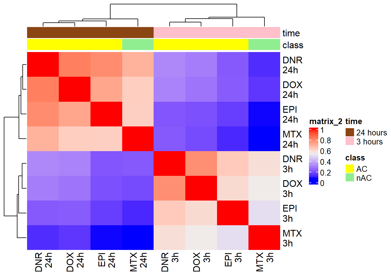
Figure S15:
Figure S15 A & B:
###now adjusted for 23 samples:
H3K27ac_counts_file <- read_delim("data/Final_four_data/H3K27ac_files/H3K27ac_counts_file.txt", delim= "\t")
PCA_H3_mat_23s <- H3K27ac_counts_file %>%
  ##removing C_VEH_3 and B_VEH_24 columns
  dplyr::select(Geneid,B_DNR_24:B_MTX_24, B_VEH_3:C_VEH_24) %>%
  column_to_rownames("Geneid") %>%
  as.matrix()

anno_H3_mat_23s <-
data.frame(timeset=colnames(PCA_H3_mat_23s)) %>%
  mutate(sample = timeset) %>%
  separate(timeset, into = c("indv","trt","time"), sep= "_") %>%
  mutate(time = factor(time, levels = c("3", "24"), labels= c("3 hours","24 hours"))) %>%
  mutate(trt = factor(trt, levels = c("DOX","EPI", "DNR", "MTX","VEH")))

for_group3 <- data.frame(timeset=colnames(PCA_H3_mat_23s)) %>%
  mutate(sample = timeset) %>%
  separate(timeset, into = c("indv","trt","time"), sep= "_") %>%
  tidyr::unite("test", trt:time,sep="_", remove = FALSE)
### for 3 individuals {2,3,6}
group_3 <- c( 1,2,4,5,6,7,10,1,2,3,4,7,8,9,10,1,2,3,5,6,7,8,9)
group_fac_3 <- group_3
groupid_3 <- as.numeric(group_fac_3)
label <- for_group3$sample
compid_3 <- data.frame(c1= c(2,4,6,8,1,3,5,7), c2 = c( 10,10,10,10,9,9,9,9))

y_TMM_cpm_3 <- cpm(PCA_H3_mat_23s, log = TRUE)

colnames(y_TMM_cpm_3) <- label

# set.seed(31415)
# cormotif_initial_3 <- cormotiffit(exprs = y_TMM_cpm_3, groupid = groupid_3, compid = compid_3, K=1:6, max.iter = 500, runtype = "logCPM")

##results from the K1:6 run:
cormotif_initial_23s <- readRDS("data/Final_four_data/cormotif_3_raodah_run_23s.RDS")

Cormotif::plotIC(cormotif_initial_23s)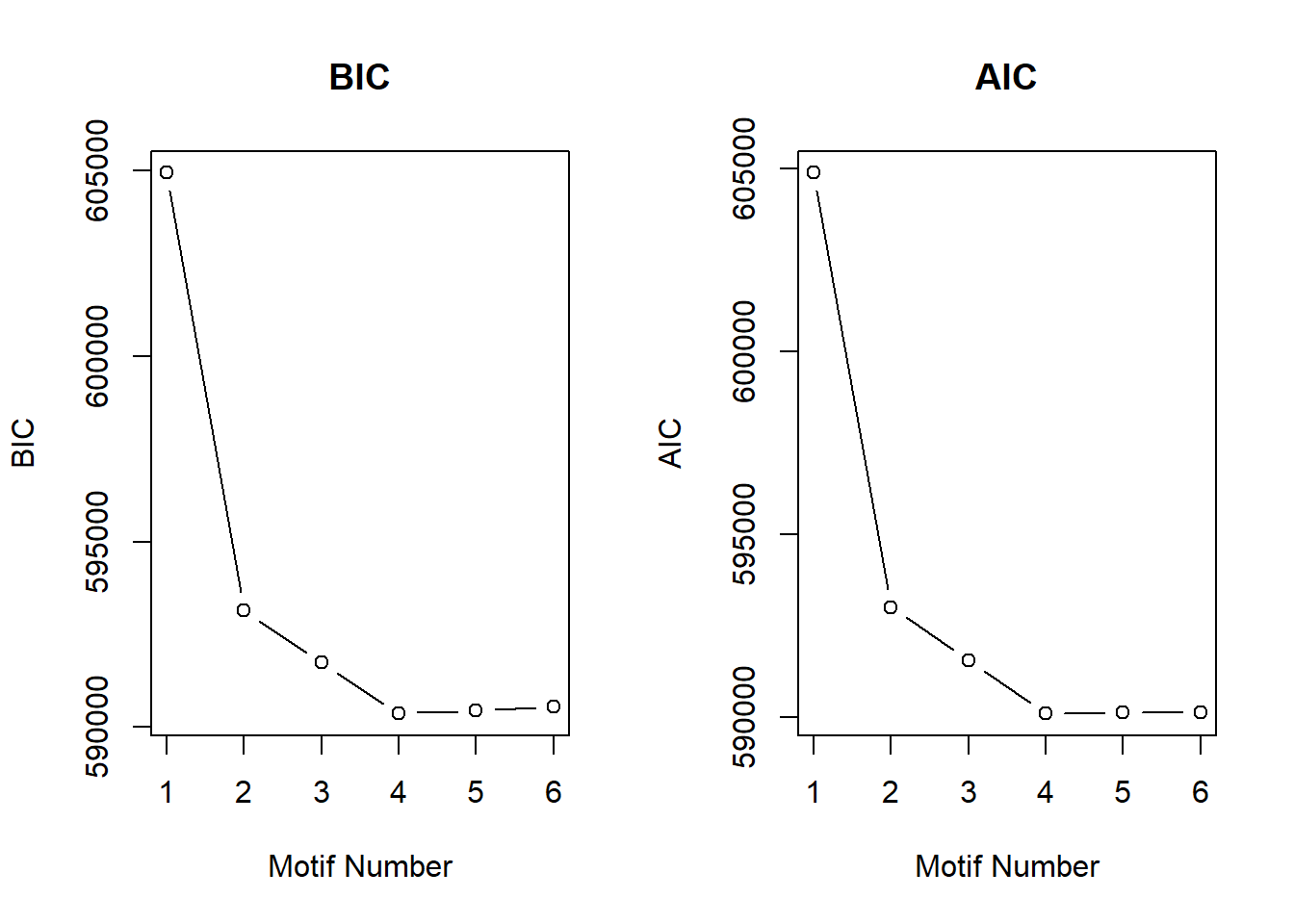
Figure S15 C:
Cormotif::plotMotif(cormotif_initial_23s)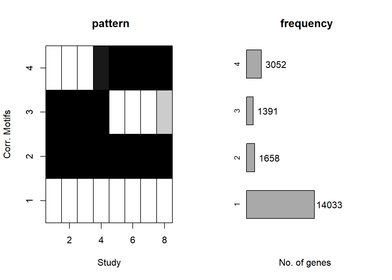
Figure S15 D:
drug_pal <- c("#8B006D","#DF707E","#F1B72B", "#3386DD","#41B333")
H3K27ac_counts_file <- read_delim("data/Final_four_data/H3K27ac_files/H3K27ac_counts_file.txt", delim= "\t")
lcpm_h3_23s <- H3K27ac_counts_file %>%
  ##removing C_VEH_3 and B_VEH_24 columns
  dplyr::select(Geneid,B_DNR_24:B_MTX_24, B_VEH_3:C_VEH_24) %>%
  column_to_rownames("Geneid") %>%
  as.matrix() %>%
 cpm(., log = TRUE)

NR_ac <- readRDS("data/Final_four_data/H3K27ac_files/NR_23s.RDS")

ESR_ac <- readRDS("data/Final_four_data/H3K27ac_files/ESR_23s.RDS")

EAR_ac <- readRDS("data/Final_four_data/H3K27ac_files/EAR_23s.RDS")

LR_ac <- readRDS("data/Final_four_data/H3K27ac_files/LR_23s.RDS")

set.seed(31415)
sample_peaks <- rbind(
  "NR_1"=sample_n(NR_ac,size = 2),
  "ESR_2"=sample_n(ESR_ac,size=2),
  "EAR_3"=sample_n(EAR_ac,size=2),
  "LR_4"=sample_n(LR_ac, size=2))
sample_peaks_choice <- sample_peaks %>%
  dplyr::filter(rownames(.)=="NR_1.2"|
                  rownames(.)=="ESR_2.1"|
                  rownames(.)=="EAR_3.1"|
                  rownames(.)=="LR_4.1")
lcpm_h3_23s%>%
  as.data.frame() %>%
  rownames_to_column("Peakid")%>%
  dplyr::filter(Peakid %in% sample_peaks_choice$Peakid) %>%
  pivot_longer(., cols = !Peakid, names_to = "samples",values_to = "logcpm") %>%
  separate_wider_delim(., samples, delim = "_",names=c("ind","trt","time"), cols_remove = FALSE) %>%
  left_join(., (sample_peaks %>%
              rownames_to_column("cluster") %>%
              dplyr::select(cluster,Peakid)),
            by=c("Peakid"="Peakid")) %>%
  mutate(trt=factor(trt, levels = c("DOX","EPI","DNR","MTX","TRZ", "VEH")),
         time= factor(time, levels = c("3","24"))) %>%
  ggplot(aes(x=time,y=logcpm))+
  geom_boxplot(aes(fill=trt))+
  # geom_point(aes(color=ind))+
  facet_wrap(~Peakid+cluster,scales="free_y", nrow=4, ncol=2)+
  ggtitle(" H3K27ac acetylation")+
  scale_fill_manual(values = drug_pal)+
  theme_bw()+
  ylab("log2 cpm H3K27ac")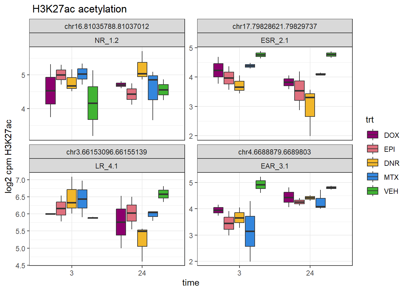
Figure S16: Shared ATAC and H3K27-acetylation regions cluster by time
toplist_atac_lfc <- readRDS("data/Final_four_data/toplist_ff.RDS")

hr3_ATAC <- toplist_atac_lfc %>%
  dplyr::select(trt:logFC) %>%
  dplyr::filter(time=="3 hours") %>%
  pivot_wider(., id_cols = c("peak"),names_from = trt,values_from = logFC) %>%
   dplyr::rename(DOX_3_ATAC=DOX, DNR_3_ATAC=DNR,EPI_3_ATAC=EPI,MTX_3_ATAC=MTX, TRZ_3_ATAC=TRZ)

hr24_ATAC <- toplist_atac_lfc %>%
  dplyr::select(trt:logFC) %>%
  dplyr::filter(time=="24 hours") %>%
  pivot_wider(., id_cols = c("peak"),names_from = trt,values_from = logFC) %>%
   dplyr::rename(DOX_24_ATAC=DOX, DNR_24_ATAC=DNR,EPI_24_ATAC=EPI,MTX_24_ATAC=MTX, TRZ_24_ATAC=TRZ)

ATAC_LFC_df <- hr3_ATAC %>%
  left_join(., hr24_ATAC, by=c("peak"="peak")) %>%
   dplyr::select(peak:MTX_3_ATAC,DNR_24_ATAC:MTX_24_ATAC)

toplist_ac_lfc <- readRDS("data/Final_four_data/toplist_ac_lfc.RDS")

hr3_K27 <- toplist_ac_lfc %>%
  dplyr::filter(time=="3") %>%
  dplyr::select(Peakid:logFC) %>%
  ###something weird in peaknames... additional numbers? so I will remove them
   mutate(Peakid=str_replace(Peakid, "\\.\\.\\.[0=9]*","/")) %>%
  separate(Peakid, into=c("Geneid",NA),sep="/") %>%
  pivot_wider(., id_cols=c(Geneid), names_from = "trt", values_from = "logFC") %>%
  dplyr::rename(DOX_3_K27=DOX, DNR_3_K27=DNR,EPI_3_K27=EPI,MTX_3_K27=MTX)

hr24_K27 <- toplist_ac_lfc %>%
  dplyr::filter(time=="24") %>%
  dplyr::select(Peakid:logFC) %>%
  ###something weird in peaknames... additional numbers? so I will remove them
   mutate(Peakid=str_replace(Peakid, "\\.\\.\\.[0=9]*","/")) %>%
  separate(Peakid, into=c("Geneid",NA),sep="/") %>%
  pivot_wider(., id_cols=c(Geneid), names_from = "trt", values_from = "logFC") %>%
  dplyr::rename(DOX_24_K27=DOX, DNR_24_K27=DNR,EPI_24_K27=EPI,MTX_24_K27=MTX)


K27_LFC_df <- hr3_K27 %>%
  left_join(., hr24_K27, by=c("Geneid"="Geneid"))


overlap_df_ggplot <- readRDS("data/Final_four_data/LFC_ATAC_K27ac.RDS") %>%
  dplyr::select(peakid,Geneid) %>%
  left_join(.,ATAC_LFC_df, by=c("peakid"="peak")) %>%
  left_join(.,K27_LFC_df, by= c("Geneid"="Geneid"))

counts_corr <-
  overlap_df_ggplot %>%
    tidyr::unite(.,"name",peakid,Geneid,sep="_") %>%
  column_to_rownames("name") %>%
  cor()
ComplexHeatmap::Heatmap(counts_corr)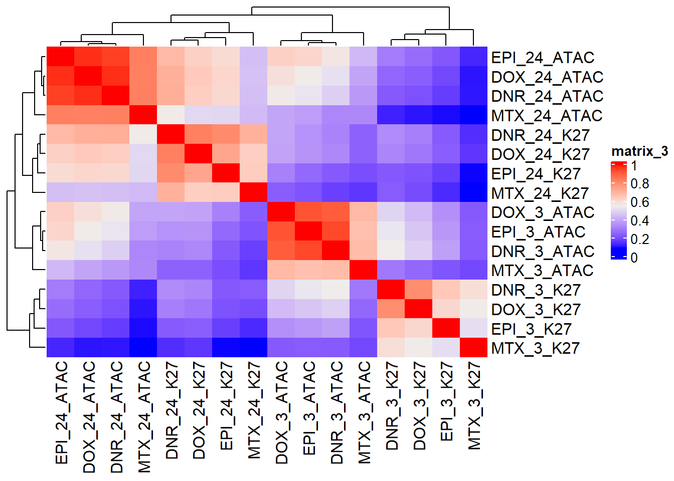
Figure S17:
RNA_ATAC_overlap_df_ggplot <- readRDS("data/Final_four_data/LFC_ATAC_K27ac.RDS") %>%
  dplyr::select(peakid,Geneid)
Collapsed_new_peaks <- read_delim("data/Final_four_data/collapsed_new_peaks.txt", delim = "\t", col_names = TRUE)

RNA_median_3_lfc <- readRDS("data/other_papers/RNA_median_3_lfc.RDS")
RNA_median_24_lfc <- readRDS("data/other_papers/RNA_median_24_lfc.RDS")
overlap_df_ggplot <- readRDS("data/Final_four_data/LFC_ATAC_K27ac.RDS")

ATAC_median_24_lfc <- read_csv("data/Final_four_data/median_24_lfc.csv")
ATAC_median_3_lfc <- read_csv("data/Final_four_data/median_3_lfc.csv")

anti_joined_lfc <- ATAC_median_24_lfc %>%
  dplyr::filter(!peak %in% RNA_ATAC_overlap_df_ggplot$peakid)  %>%
  left_join(., (Collapsed_new_peaks %>% dplyr::select(Peakid, NCBI_gene:dist_to_NG)), by = c("peak"="Peakid")) %>%
  left_join(.,ATAC_median_3_lfc,by = c("peak"="peak")) %>%
  left_join(., RNA_median_3_lfc ,
                by=c("SYMBOL"="SYMBOL", "NCBI_gene"="ENTREZID")) %>%
  left_join(., RNA_median_24_lfc,
                 by=c("SYMBOL"="SYMBOL", "NCBI_gene"="ENTREZID"))

joined_LFC_df <-
RNA_ATAC_overlap_df_ggplot %>%
  left_join(.,(Collapsed_new_peaks %>%
                 dplyr::select(Peakid,dist_to_NG, NCBI_gene:SYMBOL)),
            by=c("peakid"="Peakid")) %>%
  left_join(., RNA_median_3_lfc ,
                 by=c("SYMBOL"="SYMBOL", "NCBI_gene"="ENTREZID")) %>%
  left_join(., RNA_median_24_lfc,
             by=c("SYMBOL"="SYMBOL", "NCBI_gene"="ENTREZID")) %>%
  left_join(.,ATAC_median_3_lfc,by = c("peakid"="peak")) %>%
  left_join(.,ATAC_median_24_lfc,by = c("peakid"="peak")) %>%
  dplyr::filter(dist_to_NG > -2000| dist_to_NG <2000)


joined_LFC_df %>%
dplyr::filter(dist_to_NG>-2000 & dist_to_NG<2000) %>%
  ggplot(., aes(x=med_3h_lfc,y=RNA_3h_lfc))+
   geom_point()+
   sm_statCorr(corr_method = 'pearson')+
  ggtitle("Correlation of shared 2kb H3K27ac peaks and ATAC_peaks at 3 hours")+
  ylab("H3K27ac peak LFC")+
   xlab("ATAC-seq log FC")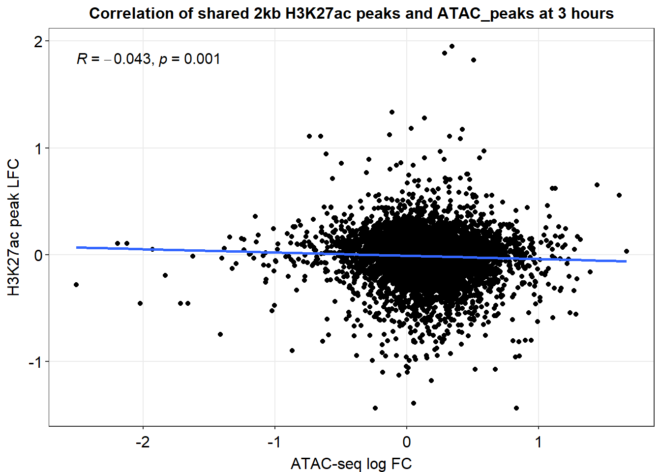
joined_LFC_df %>%
dplyr::filter(dist_to_NG>-2000 & dist_to_NG<2000) %>%
  ggplot(., aes(x=med_24h_lfc,y=RNA_24h_lfc))+
   geom_point()+
   sm_statCorr(corr_method = 'pearson')+
  ggtitle("Correlation of shared 2kb H3K27ac peaks and ATAC_peaks at 24 hours")+
  ylab("H3K27ac peak LFC")+
   xlab("ATAC-seq log FC")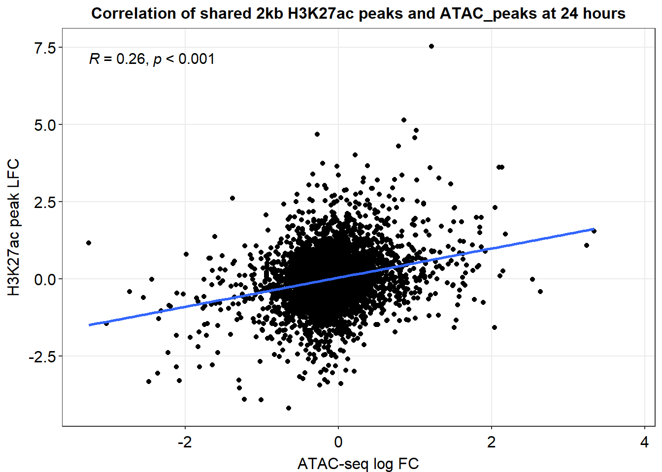
 anti_joined_lfc %>%
 dplyr::filter(dist_to_NG>-2000 & dist_to_NG<2000) %>%
   # dplyr::filter(peak %in% ATAC_LFC_df$peak) %>%
  ggplot(., aes(x=med_3h_lfc,y=RNA_3h_lfc))+
   geom_point()+
   sm_statCorr(corr_method = 'pearson')+
  ggtitle("ATAC-seq regions without H3K27ac overlap at 3 hours")+
  ylab("RNA expression LFC")+
   xlab("ATAC-seq log FC")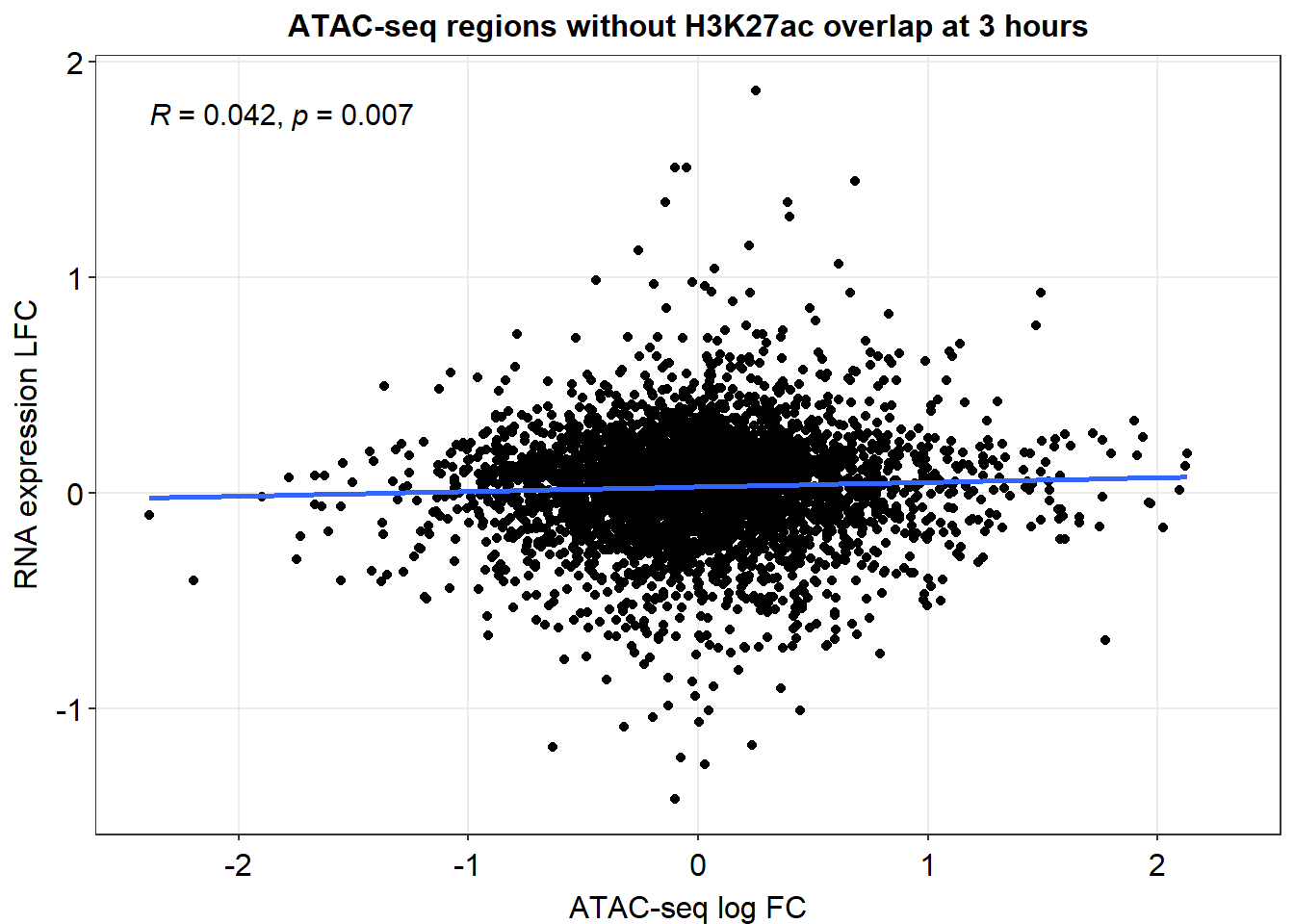
 anti_joined_lfc %>%
  dplyr::filter(dist_to_NG>-2000 & dist_to_NG<2000) %>%
ggplot(., aes(x=med_24h_lfc,y=RNA_24h_lfc))+
   geom_point()+
   sm_statCorr(corr_method = 'pearson')+
   ggtitle("Correlation of ATAC peaks not shared with H3K27ac and RNA-NG at 24 hours")+
  xlab("ATAC peak LFC")+
   ylab("RNA LFC")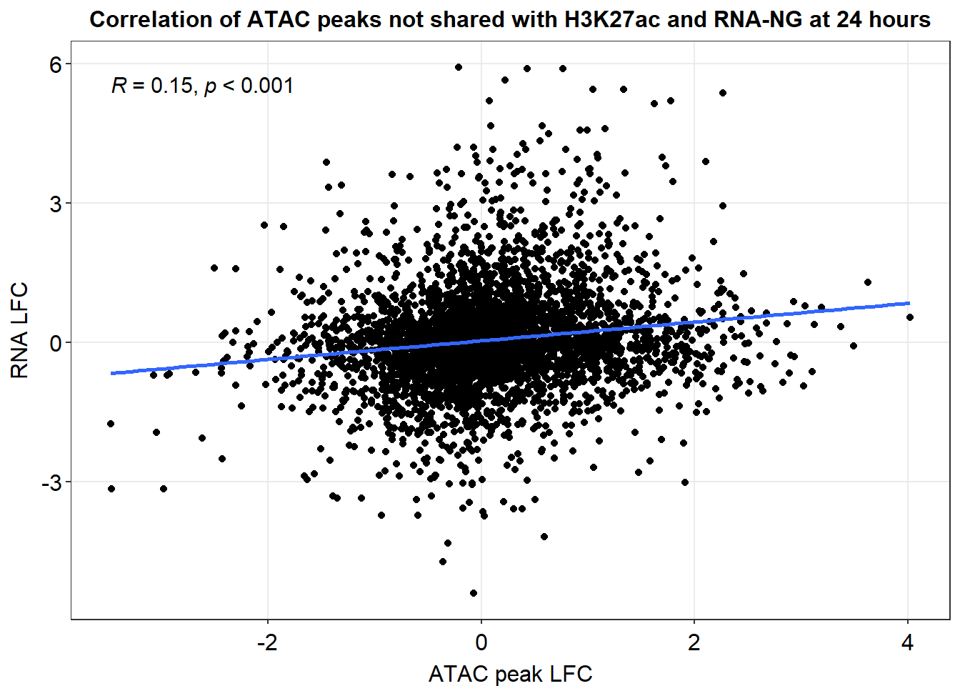
Figure S18:
toplistall_RNA <- readRDS("data/other_papers/toplistall_RNA.RDS")
toplistall_RNA <- toplistall_RNA %>%
mutate(logFC = logFC*(-1))
hr3_RNA <- toplistall_RNA %>%
dplyr::select(time:logFC) %>%
dplyr::filter(time=="3_hours") %>%
pivot_wider(., id_cols=c(ENTREZID,SYMBOL), names_from = id, values_from = logFC) %>%
dplyr::rename(DOX_3_RNA=DOX, DNR_3_RNA=DNR,EPI_3_RNA=EPI,MTX_3_RNA=MTX, TRZ_3_RNA=TRZ)
hr24_RNA <- toplistall_RNA %>%
dplyr::select(time:logFC) %>%
dplyr::filter(time=="24_hours") %>%
pivot_wider(., id_cols=c(ENTREZID,SYMBOL), names_from = id, values_from = logFC) %>%
dplyr::rename(DOX_24_RNA=DOX, DNR_24_RNA=DNR,EPI_24_RNA=EPI,MTX_24_RNA=MTX, TRZ_24_RNA=TRZ)
RNA_LFC_df <- hr3_RNA %>%
left_join(., hr24_RNA, by=c("SYMBOL"="SYMBOL","ENTREZID"="ENTREZID")) %>%
dplyr::select(ENTREZID:MTX_3_RNA,DNR_24_RNA:MTX_24_RNA)
combo_lfc <- readRDS("data/Final_four_data/LFC_ATAC_K27ac.RDS") %>%
dplyr::select(peakid,Geneid) %>%
left_join(.,ATAC_LFC_df, by=c("peakid"="peak")) %>%
left_join(.,K27_LFC_df, by= c("Geneid"="Geneid"))
combo_corr <- combo_lfc %>%
left_join(.,(Collapsed_new_peaks %>%
dplyr::select(Peakid, NCBI_gene,SYMBOL)), by=c("peakid"="Peakid")) %>%
left_join(., RNA_LFC_df, by=c("SYMBOL"="SYMBOL","NCBI_gene"="ENTREZID")) %>%
tidyr::unite(., "name",peakid,Geneid,NCBI_gene,SYMBOL,sep = "_") %>%
column_to_rownames("name") %>%
na.omit() %>%
cor()
ComplexHeatmap::Heatmap(combo_corr)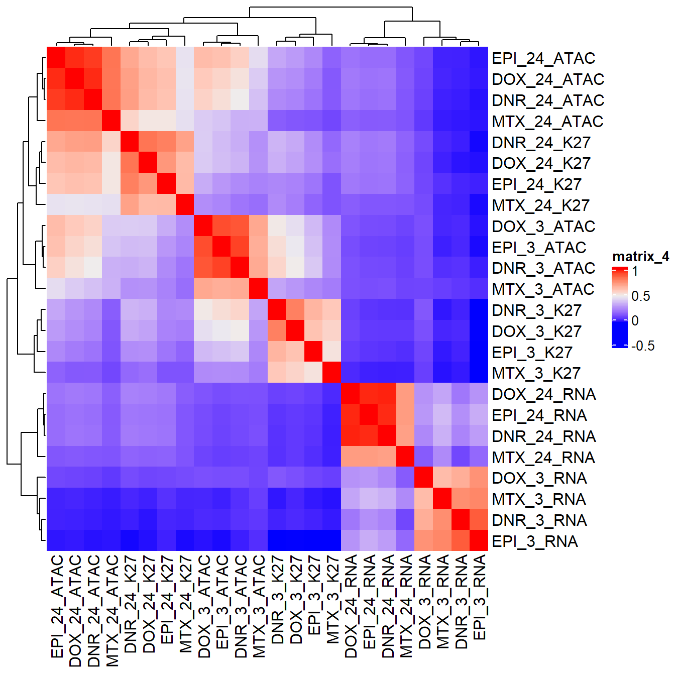 ###: Figure S19
drug_pal <- c("#8B006D","#DF707E","#F1B72B", "#3386DD","#707031","#41B333")
PRDX6_info <- Collapsed_new_peaks %>% dplyr::filter(SYMBOL=="PRDX6") %>%
  distinct(NCBI_gene,SYMBOL)

RNA_counts <- readRDS("data/other_papers/cpmcount.RDS") %>%
  dplyr::rename_with(.,~gsub(pattern="Da",replacement="DNR",.)) %>%
 dplyr::rename_with(.,~gsub(pattern="Do",replacement="DOX",.)) %>%
  dplyr::rename_with(.,~gsub(pattern="Ep",replacement="EPI",.)) %>%
   dplyr::rename_with(.,~gsub(pattern="Mi",replacement="MTX",.)) %>%
    dplyr::rename_with(.,~gsub(pattern="Tr",replacement="TRZ",.)) %>%
       dplyr::rename_with(.,~gsub(pattern="Ve",replacement="VEH",.)) %>%
  rownames_to_column("ENTREZID")


RNA_counts %>%
  dplyr::filter(ENTREZID == PRDX6_info$NCBI_gene) %>%
  pivot_longer(cols = !ENTREZID, names_to = "sample", values_to = "counts") %>%
  left_join(., PRDX6_info, by =c("ENTREZID"="NCBI_gene")) %>%
  separate("sample", into = c("trt","ind","time")) %>%
  mutate(time=factor(time, levels = c("3h","24h"))) %>%
  mutate(trt=factor(trt, levels= c("DOX","EPI","DNR","MTX","TRZ","VEH"))) %>%
  ggplot(., aes (x = time, y=counts))+
  geom_boxplot(aes(fill=trt))+
  facet_wrap(~SYMBOL, scales="free_y")+
  ggtitle("RNA log 2 cpm of expressed gene")+
    scale_fill_manual(values = drug_pal)+
  theme_bw()+
  ylab("log2 cpm RNA")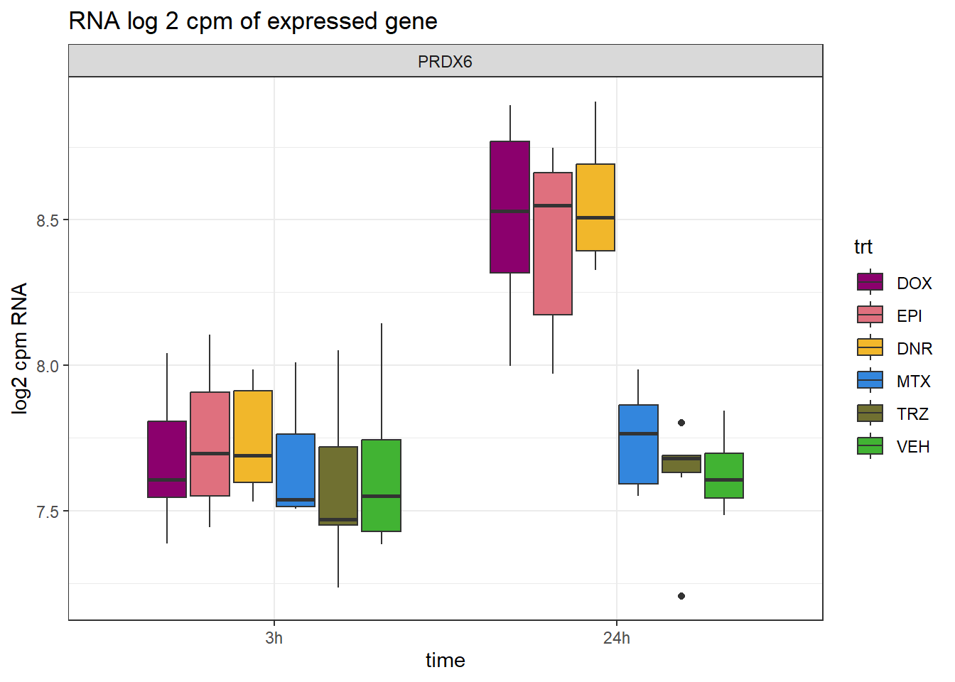
PRUNE2_info <- Collapsed_new_peaks %>% dplyr::filter(SYMBOL=="PRUNE2") %>%
  distinct(NCBI_gene,SYMBOL)


RNA_counts %>%
  dplyr::filter(ENTREZID == PRUNE2_info$NCBI_gene) %>%
  pivot_longer(cols = !ENTREZID, names_to = "sample", values_to = "counts") %>%
  left_join(., PRUNE2_info, by =c("ENTREZID"="NCBI_gene")) %>%
  separate("sample", into = c("trt","ind","time")) %>%
  mutate(time=factor(time, levels = c("3h","24h"))) %>%
  mutate(trt=factor(trt, levels= c("DOX","EPI","DNR","MTX","TRZ","VEH"))) %>%
  ggplot(., aes (x = time, y=counts))+
  geom_boxplot(aes(fill=trt))+
  facet_wrap(~SYMBOL, scales="free_y")+
  ggtitle("RNA log 2 cpm of expressed gene")+
    scale_fill_manual(values = drug_pal)+
  theme_bw()+
  ylab("log2 cpm RNA")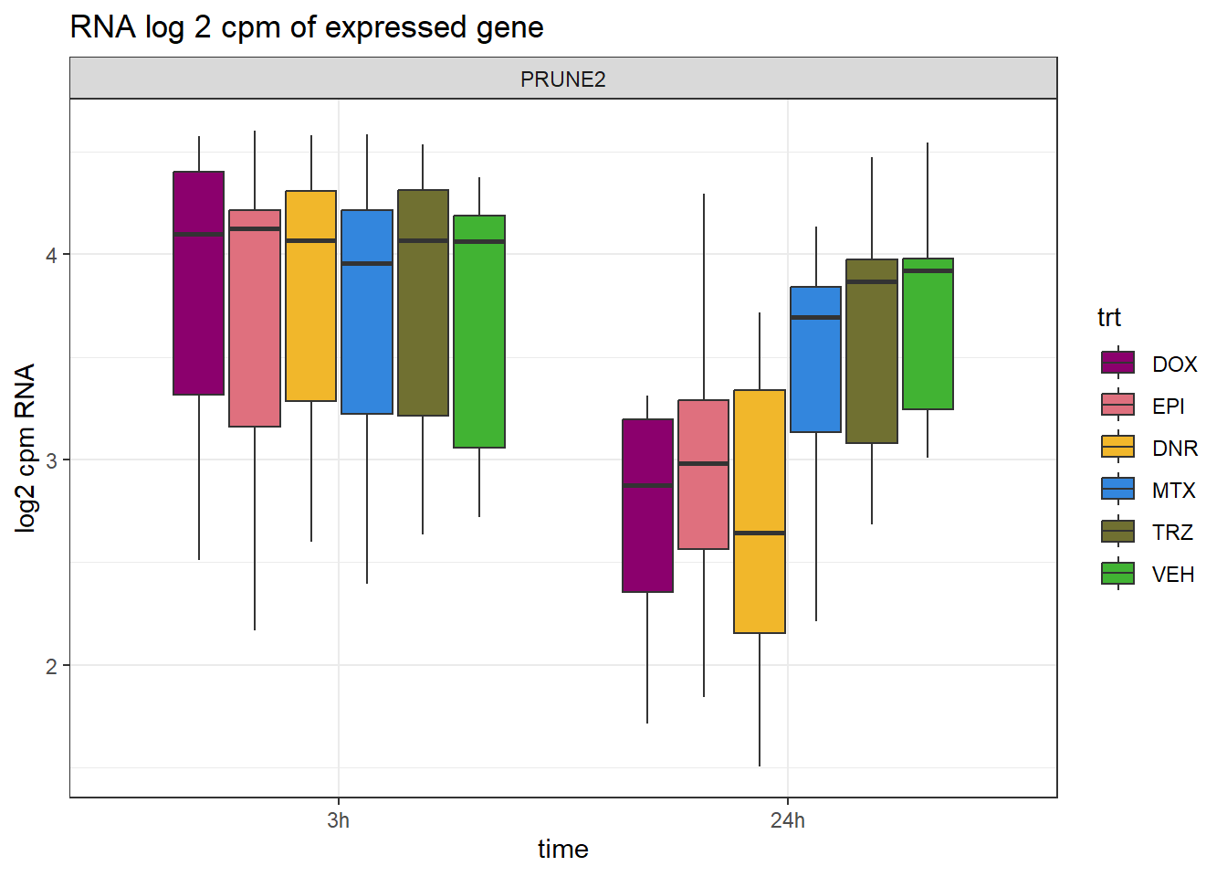
sessionInfo()R version 4.4.2 (2024-10-31 ucrt)
Platform: x86_64-w64-mingw32/x64
Running under: Windows 11 x64 (build 26100)
Matrix products: default
locale:
[1] LC_COLLATE=English_United States.utf8
[2] LC_CTYPE=English_United States.utf8
[3] LC_MONETARY=English_United States.utf8
[4] LC_NUMERIC=C
[5] LC_TIME=English_United States.utf8
time zone: America/Chicago
tzcode source: internal
attached base packages:
[1] grid stats4 stats graphics grDevices utils datasets
[8] methods base
other attached packages:
[1] eulerr_7.0.2
[2] vargen_0.2.3
[3] devtools_2.4.5
[4] usethis_3.1.0
[5] readxl_1.4.3
[6] smplot2_0.2.5
[7] cowplot_1.1.3
[8] ComplexHeatmap_2.22.0
[9] ggrepel_0.9.6
[10] plyranges_1.26.0
[11] ggsignif_0.6.4
[12] genomation_1.38.0
[13] edgeR_4.4.1
[14] limma_3.62.2
[15] ggpubr_0.6.0
[16] BiocParallel_1.40.0
[17] ggVennDiagram_1.5.2
[18] scales_1.3.0
[19] VennDiagram_1.7.3
[20] futile.logger_1.4.3
[21] gridExtra_2.3
[22] ggfortify_0.4.17
[23] rtracklayer_1.66.0
[24] org.Hs.eg.db_3.20.0
[25] TxDb.Hsapiens.UCSC.hg38.knownGene_3.20.0
[26] GenomicFeatures_1.58.0
[27] AnnotationDbi_1.68.0
[28] Biobase_2.66.0
[29] GenomicRanges_1.58.0
[30] GenomeInfoDb_1.42.1
[31] IRanges_2.40.1
[32] S4Vectors_0.44.0
[33] BiocGenerics_0.52.0
[34] ChIPseeker_1.42.0
[35] RColorBrewer_1.1-3
[36] broom_1.0.7
[37] kableExtra_1.4.0
[38] lubridate_1.9.4
[39] forcats_1.0.0
[40] stringr_1.5.1
[41] dplyr_1.1.4
[42] purrr_1.0.2
[43] readr_2.1.5
[44] tidyr_1.3.1
[45] tibble_3.2.1
[46] ggplot2_3.5.1
[47] tidyverse_2.0.0
[48] workflowr_1.7.1
loaded via a namespace (and not attached):
[1] fs_1.6.5
[2] matrixStats_1.5.0
[3] bitops_1.0-9
[4] enrichplot_1.26.6
[5] httr_1.4.7
[6] doParallel_1.0.17
[7] profvis_0.4.0
[8] tools_4.4.2
[9] backports_1.5.0
[10] R6_2.5.1
[11] mgcv_1.9-1
[12] lazyeval_0.2.2
[13] GetoptLong_1.0.5
[14] urlchecker_1.0.1
[15] withr_3.0.2
[16] preprocessCore_1.68.0
[17] cli_3.6.3
[18] formatR_1.14
[19] Cormotif_1.52.0
[20] labeling_0.4.3
[21] sass_0.4.9
[22] Rsamtools_2.22.0
[23] systemfonts_1.2.1
[24] yulab.utils_0.2.0
[25] foreign_0.8-88
[26] DOSE_4.0.0
[27] svglite_2.1.3
[28] R.utils_2.12.3
[29] sessioninfo_1.2.2
[30] plotrix_3.8-4
[31] BSgenome_1.74.0
[32] pwr_1.3-0
[33] rstudioapi_0.17.1
[34] impute_1.80.0
[35] RSQLite_2.3.9
[36] generics_0.1.3
[37] gridGraphics_0.5-1
[38] TxDb.Hsapiens.UCSC.hg19.knownGene_3.2.2
[39] shape_1.4.6.1
[40] BiocIO_1.16.0
[41] vroom_1.6.5
[42] gtools_3.9.5
[43] car_3.1-3
[44] GO.db_3.20.0
[45] Matrix_1.7-2
[46] abind_1.4-8
[47] R.methodsS3_1.8.2
[48] lifecycle_1.0.4
[49] whisker_0.4.1
[50] yaml_2.3.10
[51] carData_3.0-5
[52] SummarizedExperiment_1.36.0
[53] gplots_3.2.0
[54] qvalue_2.38.0
[55] SparseArray_1.6.1
[56] blob_1.2.4
[57] promises_1.3.2
[58] crayon_1.5.3
[59] miniUI_0.1.1.1
[60] ggtangle_0.0.6
[61] lattice_0.22-6
[62] KEGGREST_1.46.0
[63] magick_2.8.5
[64] pillar_1.10.1
[65] knitr_1.49
[66] fgsea_1.32.2
[67] rjson_0.2.23
[68] boot_1.3-31
[69] codetools_0.2-20
[70] fastmatch_1.1-6
[71] glue_1.8.0
[72] getPass_0.2-4
[73] ggfun_0.1.8
[74] remotes_2.5.0
[75] data.table_1.16.4
[76] vctrs_0.6.5
[77] png_0.1-8
[78] treeio_1.30.0
[79] cellranger_1.1.0
[80] gtable_0.3.6
[81] cachem_1.1.0
[82] xfun_0.50
[83] mime_0.12
[84] S4Arrays_1.6.0
[85] iterators_1.0.14
[86] statmod_1.5.0
[87] ellipsis_0.3.2
[88] nlme_3.1-167
[89] ggtree_3.14.0
[90] bit64_4.6.0-1
[91] rprojroot_2.0.4
[92] bslib_0.8.0
[93] affyio_1.76.0
[94] rpart_4.1.24
[95] KernSmooth_2.23-26
[96] colorspace_2.1-1
[97] DBI_1.2.3
[98] Hmisc_5.2-2
[99] nnet_7.3-20
[100] seqPattern_1.38.0
[101] tidyselect_1.2.1
[102] processx_3.8.5
[103] bit_4.5.0.1
[104] compiler_4.4.2
[105] curl_6.2.0
[106] git2r_0.35.0
[107] htmlTable_2.4.3
[108] xml2_1.3.6
[109] DelayedArray_0.32.0
[110] checkmate_2.3.2
[111] caTools_1.18.3
[112] affy_1.84.0
[113] callr_3.7.6
[114] digest_0.6.37
[115] rmarkdown_2.29
[116] XVector_0.46.0
[117] htmltools_0.5.8.1
[118] pkgconfig_2.0.3
[119] base64enc_0.1-3
[120] MatrixGenerics_1.18.1
[121] fastmap_1.2.0
[122] htmlwidgets_1.6.4
[123] rlang_1.1.5
[124] GlobalOptions_0.1.2
[125] UCSC.utils_1.2.0
[126] shiny_1.10.0
[127] farver_2.1.2
[128] jquerylib_0.1.4
[129] zoo_1.8-12
[130] jsonlite_1.8.9
[131] GOSemSim_2.32.0
[132] R.oo_1.27.0
[133] RCurl_1.98-1.16
[134] magrittr_2.0.3
[135] Formula_1.2-5
[136] GenomeInfoDbData_1.2.13
[137] ggplotify_0.1.2
[138] patchwork_1.3.0
[139] munsell_0.5.1
[140] Rcpp_1.0.14
[141] ape_5.8-1
[142] stringi_1.8.4
[143] zlibbioc_1.52.0
[144] pkgbuild_1.4.6
[145] plyr_1.8.9
[146] parallel_4.4.2
[147] Biostrings_2.74.1
[148] splines_4.4.2
[149] hms_1.1.3
[150] circlize_0.4.16
[151] locfit_1.5-9.10
[152] ps_1.8.1
[153] igraph_2.1.4
[154] pkgload_1.4.0
[155] reshape2_1.4.4
[156] futile.options_1.0.1
[157] XML_3.99-0.18
[158] evaluate_1.0.3
[159] BiocManager_1.30.25
[160] lambda.r_1.2.4
[161] tzdb_0.4.0
[162] foreach_1.5.2
[163] httpuv_1.6.15
[164] clue_0.3-66
[165] gridBase_0.4-7
[166] xtable_1.8-4
[167] restfulr_0.0.15
[168] tidytree_0.4.6
[169] rstatix_0.7.2
[170] later_1.4.1
[171] viridisLite_0.4.2
[172] aplot_0.2.4
[173] memoise_2.0.1
[174] GenomicAlignments_1.42.0
[175] cluster_2.1.8
[176] timechange_0.3.0