Peak_analysis
ERM
2024-03-08
Last updated: 2024-03-08
Checks: 7 0
Knit directory: ATAC_learning/
This reproducible R Markdown analysis was created with workflowr (version 1.7.1). The Checks tab describes the reproducibility checks that were applied when the results were created. The Past versions tab lists the development history.
Great! Since the R Markdown file has been committed to the Git repository, you know the exact version of the code that produced these results.
Great job! The global environment was empty. Objects defined in the global environment can affect the analysis in your R Markdown file in unknown ways. For reproduciblity it’s best to always run the code in an empty environment.
The command set.seed(20231016) was run prior to running
the code in the R Markdown file. Setting a seed ensures that any results
that rely on randomness, e.g. subsampling or permutations, are
reproducible.
Great job! Recording the operating system, R version, and package versions is critical for reproducibility.
Nice! There were no cached chunks for this analysis, so you can be confident that you successfully produced the results during this run.
Great job! Using relative paths to the files within your workflowr project makes it easier to run your code on other machines.
Great! You are using Git for version control. Tracking code development and connecting the code version to the results is critical for reproducibility.
The results in this page were generated with repository version 7906ccf. See the Past versions tab to see a history of the changes made to the R Markdown and HTML files.
Note that you need to be careful to ensure that all relevant files for
the analysis have been committed to Git prior to generating the results
(you can use wflow_publish or
wflow_git_commit). workflowr only checks the R Markdown
file, but you know if there are other scripts or data files that it
depends on. Below is the status of the Git repository when the results
were generated:
Ignored files:
    Ignored:    .Rhistory
    Ignored:    .Rproj.user/
    Ignored:    analysis/figure/
    Ignored:    data/All_merged_peaks.tsv
    Ignored:    data/Ind1_75DA24h_dedup_peaks.csv
    Ignored:    data/Ind1_TSS_peaks.RDS
    Ignored:    data/Ind1_firstfragment_files.txt
    Ignored:    data/Ind1_fragment_files.txt
    Ignored:    data/Ind1_peaks_list.RDS
    Ignored:    data/Ind1_summary.txt
    Ignored:    data/Ind2_TSS_peaks.RDS
    Ignored:    data/Ind2_fragment_files.txt
    Ignored:    data/Ind2_peaks_list.RDS
    Ignored:    data/Ind2_summary.txt
    Ignored:    data/Ind3_TSS_peaks.RDS
    Ignored:    data/Ind3_fragment_files.txt
    Ignored:    data/Ind3_peaks_list.RDS
    Ignored:    data/Ind3_summary.txt
    Ignored:    data/Ind4_79B24h_dedup_peaks.csv
    Ignored:    data/Ind4_TSS_peaks.RDS
    Ignored:    data/Ind4_V24h_fraglength.txt
    Ignored:    data/Ind4_fragment_files.txt
    Ignored:    data/Ind4_fragment_filesN.txt
    Ignored:    data/Ind4_peaks_list.RDS
    Ignored:    data/Ind4_summary.txt
    Ignored:    data/Ind5_TSS_peaks.RDS
    Ignored:    data/Ind5_fragment_files.txt
    Ignored:    data/Ind5_fragment_filesN.txt
    Ignored:    data/Ind5_peaks_list.RDS
    Ignored:    data/Ind5_summary.txt
    Ignored:    data/Ind6_TSS_peaks.RDS
    Ignored:    data/Ind6_fragment_files.txt
    Ignored:    data/Ind6_peaks_list.RDS
    Ignored:    data/Ind6_summary.txt
    Ignored:    data/aln_run1_results.txt
    Ignored:    data/anno_ind1_DA24h.RDS
    Ignored:    data/anno_ind4_V24h.RDS
    Ignored:    data/first_Peaksummarycounts.csv
    Ignored:    data/first_run_frag_counts.txt
    Ignored:    data/ind1_DA24hpeaks.RDS
    Ignored:    data/ind4_V24hpeaks.RDS
    Ignored:    data/initial_complete_stats_run1.txt
    Ignored:    data/mergedPeads.gff
    Ignored:    data/mergedPeaks.gff
    Ignored:    data/multiqc_fastqc_run1.txt
    Ignored:    data/multiqc_fastqc_run2.txt
    Ignored:    data/multiqc_genestat_run1.txt
    Ignored:    data/multiqc_genestat_run2.txt
    Ignored:    data/peakAnnoList_1.RDS
    Ignored:    data/peakAnnoList_2.RDS
    Ignored:    data/peakAnnoList_3.RDS
    Ignored:    data/peakAnnoList_4.RDS
    Ignored:    data/peakAnnoList_5.RDS
    Ignored:    data/peakAnnoList_6.RDS
    Ignored:    data/trimmed_seq_length.csv

Untracked files:
    Untracked:  Firstcorr plotATAC.pdf
    Untracked:  code/just_for_Fun.R
    Untracked:  lcpm_filtered_corplot.pdf
    Untracked:  log2cpmfragcount.pdf
    Untracked:  splited/
Note that any generated files, e.g. HTML, png, CSS, etc., are not included in this status report because it is ok for generated content to have uncommitted changes.
These are the previous versions of the repository in which changes were
made to the R Markdown (analysis/Peak_analysis.Rmd) and
HTML (docs/Peak_analysis.html) files. If you’ve configured
a remote Git repository (see ?wflow_git_remote), click on
the hyperlinks in the table below to view the files as they were in that
past version.
| File | Version | Author | Date | Message |
|---|---|---|---|---|
| Rmd | 7906ccf | reneeisnowhere | 2024-03-08 | adding new page |
library(tidyverse)
# library(ggsignif)
# library(cowplot)
# library(ggpubr)
# library(scales)
# library(sjmisc)
library(kableExtra)
# library(broom)
# library(biomaRt)
library(RColorBrewer)
# library(gprofiler2)
# library(qvalue)
# library(ChIPseeker)
# library("TxDb.Hsapiens.UCSC.hg38.knownGene")
# library("org.Hs.eg.db")
# library(ATACseqQC)
# library(rtracklayer)
library(edgeR)
library(ggfortify)
pca_plot <-
function(df,
col_var = NULL,
shape_var = NULL,
title = "") {
ggplot(df) + geom_point(aes_string(
x = "PC1",
y = "PC2",
color = col_var,
shape = shape_var
),
size = 5) +
labs(title = title, x = "PC 1", y = "PC 2") +
scale_color_manual(values = c(
"#8B006D",
"#DF707E",
"#F1B72B",
"#3386DD",
"#707031",
"#41B333"
))
}
pca_var_plot <- function(pca) {
# x: class == prcomp
pca.var <- pca$sdev ^ 2
pca.prop <- pca.var / sum(pca.var)
var.plot <-
qplot(PC, prop, data = data.frame(PC = 1:length(pca.prop),
prop = pca.prop)) +
labs(title = 'Variance contributed by each PC',
x = 'PC', y = 'Proportion of variance')
}
calc_pca <- function(x) {
# Performs principal components analysis with prcomp
# x: a sample-by-gene numeric matrix
prcomp(x, scale. = TRUE, retx = TRUE)
}
get_regr_pval <- function(mod) {
# Returns the p-value for the Fstatistic of a linear model
# mod: class lm
stopifnot(class(mod) == "lm")
fstat <- summary(mod)$fstatistic
pval <- 1 - pf(fstat[1], fstat[2], fstat[3])
return(pval)
}
plot_versus_pc <- function(df, pc_num, fac) {
# df: data.frame
# pc_num: numeric, specific PC for plotting
# fac: column name of df for plotting against PC
pc_char <- paste0("PC", pc_num)
# Calculate F-statistic p-value for linear model
pval <- get_regr_pval(lm(df[, pc_char] ~ df[, fac]))
if (is.numeric(df[, f])) {
ggplot(df, aes_string(x = f, y = pc_char)) + geom_point() +
geom_smooth(method = "lm") + labs(title = sprintf("p-val: %.2f", pval))
} else {
ggplot(df, aes_string(x = f, y = pc_char)) + geom_boxplot() +
labs(title = sprintf("p-val: %.2f", pval))
}
}
x_axis_labels = function(labels, every_nth = 1, ...) {
axis(side = 1,
at = seq_along(labels),
labels = F)
text(
x = (seq_along(labels))[seq_len(every_nth) == 1],
y = par("usr")[3] - 0.075 * (par("usr")[4] - par("usr")[3]),
labels = labels[seq_len(every_nth) == 1],
xpd = TRUE,
...
)
}first_run_frag_counts <- read.csv("data/first_run_frag_counts.txt", row.names = 1)
Frag_cor <- first_run_frag_counts %>%
dplyr::select(Ind1_75DA24h:Ind6_71V3h) %>%
cpm(., log = TRUE) %>%
cor()
filmat_groupmat_col <- data.frame(timeset = colnames(Frag_cor))
counts_corr_mat <-filmat_groupmat_col %>%
mutate(timeset=gsub("75","1_",timeset)) %>%
mutate(timeset=gsub("87","2_",timeset)) %>%
mutate(timeset=gsub("77","3_",timeset)) %>%
mutate(timeset=gsub("79","4_",timeset)) %>%
mutate(timeset=gsub("78","5_",timeset)) %>%
mutate(timeset=gsub("71","6_",timeset)) %>%
mutate(timeset = gsub("24h","_24h",timeset),
timeset = gsub("3h","_3h",timeset)) %>%
separate(timeset, into = c(NA,"indv","trt","time"), sep= "_") %>%
mutate(trt= case_match(trt, 'DX' ~'DOX', 'E'~'EPI', 'DA'~'DNR', 'M'~'MTX', 'T'~'TRZ', 'V'~'VEH',.default = trt)) %>%
mutate(class = if_else(trt == "DNR", "AC", if_else(
trt == "DOX", "AC", if_else(trt == "EPI", "AC", "nAC")
))) %>%
mutate(TOP2i = if_else(trt == "DNR", "yes", if_else(
trt == "DOX", "yes", if_else(trt == "EPI", "yes", if_else(trt == "MTX", "yes", "no"))
)))
mat_colors <- list(
trt= c("#F1B72B","#8B006D","#DF707E","#3386DD","#707031","#41B333"),
indv=c("#1B9E77", "#D95F02" ,"#7570B3", "#E7298A" ,"#66A61E", "#E6AB02"),
time=c("pink", "chocolate4"),
class=c("yellow1","darkorange1"),
TOP2i =c("darkgreen","lightgreen"))
names(mat_colors$trt) <- unique(counts_corr_mat$trt)
names(mat_colors$indv) <- unique(counts_corr_mat$indv)
names(mat_colors$time) <- unique(counts_corr_mat$time)
names(mat_colors$class) <- unique(counts_corr_mat$class)
names(mat_colors$TOP2i) <- unique(counts_corr_mat$TOP2i)
ComplexHeatmap::pheatmap(Frag_cor,
# column_title=(paste0("RNA-seq log"[2]~"cpm correlation")),
annotation_col = counts_corr_mat,
annotation_colors = mat_colors,
heatmap_legend_param = mat_colors,
fontsize=10,
fontsize_row = 8,
angle_col="90",
treeheight_row=25,
fontsize_col = 8,
treeheight_col = 20)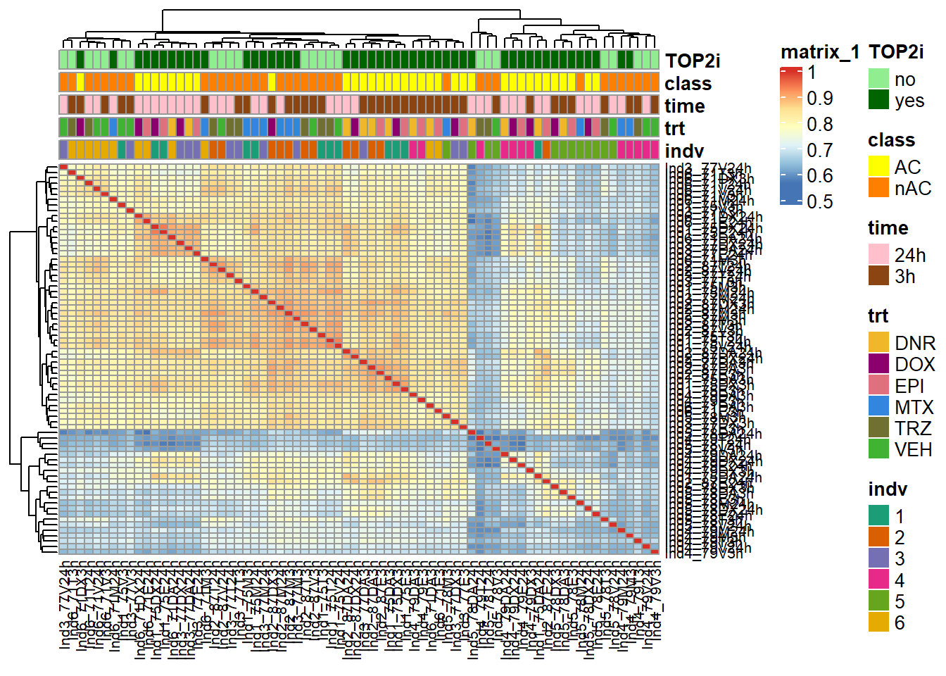
first_run_frag_counts <- read.csv("data/first_run_frag_counts.txt", row.names = 1)

##loading of the counts matrix
##then separting off the non-counts columns
PCAmat <- first_run_frag_counts %>%
  dplyr::select(Ind1_75DA24h:Ind6_71V3h) %>% as.matrix()

annotation_mat <- data.frame(timeset=colnames(PCAmat)) %>%
  mutate(sample = timeset) %>%
  mutate(timeset=gsub("Ind1_75","1_",timeset)) %>%
  mutate(timeset=gsub("Ind2_87","2_",timeset)) %>%
  mutate(timeset=gsub("Ind3_77","3_",timeset)) %>%
  mutate(timeset=gsub("Ind4_79","4_",timeset)) %>%
  mutate(timeset=gsub("Ind5_78","5_",timeset)) %>%
  mutate(timeset=gsub("Ind6_71","6_",timeset)) %>%
  mutate(timeset = gsub("24h","_24h",timeset),
       timeset = gsub("3h","_3h",timeset)) %>%
  separate(timeset, into = c("indv","trt","time"), sep= "_") %>%
  mutate(trt= case_match(trt, 'DX' ~'DOX', 'E'~'EPI', 'DA'~'DNR', 'M'~'MTX', 'T'~'TRZ', 'V'~'VEH',.default = trt)) %>%
  # mutate(indv = factor(indv, levels = c("1", "2", "3", "4", "5", "6"))) %>%
  mutate(time = factor(time, levels = c("3h", "24h"), labels= c("3 hours","24 hours"))) %>%
  mutate(trt = factor(trt, levels = c("DOX","EPI", "DNR", "MTX", "TRZ", "VEH")))

PCA_info <- (prcomp(t(PCAmat), scale. = TRUE))
PCA_info_anno <- PCA_info$x %>% cbind(.,annotation_mat)
# autoplot(PCA_info)
summary(PCA_info)
Importance of components:
PC1 PC2 PC3 PC4 PC5
Standard deviation 376.9018 203.90212 167.84380 130.89150 111.62091
Proportion of Variance 0.3062 0.08961 0.06072 0.03693 0.02685
Cumulative Proportion 0.3062 0.39580 0.45652 0.49345 0.52031
PC6 PC7 PC8 PC9 PC10 PC11
Standard deviation 98.43631 92.6486 84.97646 81.63429 79.45811 77.59140
Proportion of Variance 0.02089 0.0185 0.01556 0.01436 0.01361 0.01298
Cumulative Proportion 0.54119 0.5597 0.57526 0.58962 0.60323 0.61621
PC12 PC13 PC14 PC15 PC16 PC17
Standard deviation 74.48303 73.59252 71.32544 68.95613 67.61537 66.62440
Proportion of Variance 0.01196 0.01167 0.01097 0.01025 0.00985 0.00957
Cumulative Proportion 0.62816 0.63984 0.65080 0.66105 0.67091 0.68047
PC18 PC19 PC20 PC21 PC22 PC23
Standard deviation 65.89180 65.52139 65.01338 64.59942 63.83943 62.55323
Proportion of Variance 0.00936 0.00925 0.00911 0.00899 0.00878 0.00843
Cumulative Proportion 0.68983 0.69908 0.70820 0.71719 0.72597 0.73441
PC24 PC25 PC26 PC27 PC28 PC29
Standard deviation 62.11037 61.85108 61.03154 60.79074 60.08203 59.53870
Proportion of Variance 0.00831 0.00825 0.00803 0.00797 0.00778 0.00764
Cumulative Proportion 0.74272 0.75097 0.75900 0.76696 0.77474 0.78238
PC30 PC31 PC32 PC33 PC34 PC35
Standard deviation 59.28043 58.34606 57.34933 56.48724 55.83691 55.01438
Proportion of Variance 0.00757 0.00734 0.00709 0.00688 0.00672 0.00652
Cumulative Proportion 0.78996 0.79730 0.80439 0.81126 0.81798 0.82451
PC36 PC37 PC38 PC39 PC40 PC41
Standard deviation 53.98905 53.89602 53.55217 53.14725 52.91971 52.68384
Proportion of Variance 0.00628 0.00626 0.00618 0.00609 0.00604 0.00598
Cumulative Proportion 0.83079 0.83705 0.84323 0.84932 0.85536 0.86134
PC42 PC43 PC44 PC45 PC46 PC47
Standard deviation 52.40497 52.08406 51.99267 51.63864 51.4089 50.93515
Proportion of Variance 0.00592 0.00585 0.00583 0.00575 0.0057 0.00559
Cumulative Proportion 0.86726 0.87311 0.87893 0.88468 0.8904 0.89597
PC48 PC49 PC50 PC51 PC52 PC53
Standard deviation 50.46722 50.23329 49.78971 49.54472 48.6485 48.33228
Proportion of Variance 0.00549 0.00544 0.00534 0.00529 0.0051 0.00504
Cumulative Proportion 0.90146 0.90690 0.91224 0.91753 0.9226 0.92767
PC54 PC55 PC56 PC57 PC58 PC59
Standard deviation 48.22246 47.52685 47.33857 46.97043 46.7177 46.25328
Proportion of Variance 0.00501 0.00487 0.00483 0.00476 0.0047 0.00461
Cumulative Proportion 0.93268 0.93755 0.94238 0.94713 0.9518 0.95645
PC60 PC61 PC62 PC63 PC64 PC65
Standard deviation 45.96486 45.31000 45.12708 44.1664 43.29335 42.38188
Proportion of Variance 0.00455 0.00443 0.00439 0.0042 0.00404 0.00387
Cumulative Proportion 0.96100 0.96543 0.96982 0.9740 0.97806 0.98193
PC66 PC67 PC68 PC69 PC70 PC71
Standard deviation 41.31984 40.12882 38.78887 35.99534 34.36816 32.90725
Proportion of Variance 0.00368 0.00347 0.00324 0.00279 0.00255 0.00233
Cumulative Proportion 0.98561 0.98908 0.99233 0.99512 0.99767 1.00000
PC72
Standard deviation 1.156e-12
Proportion of Variance 0.000e+00
Cumulative Proportion 1.000e+00# cpm(PCAmat, log=TRUE)
pca_plot(PCA_info_anno, col_var='trt', shape_var = 'time')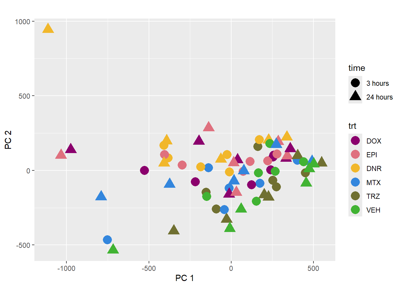
pca_plot(PCA_info_anno, col_var='trt', shape_var = 'indv')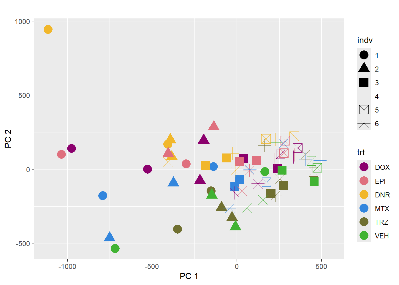
lcpm <- cpm(PCAmat, log=TRUE)  ### for determining the basic cutoffs
dim(lcpm)
[1] 463947 72row_means <- rowMeans(lcpm)
x_filtered <- PCAmat[row_means > 0,]
dim(x_filtered)[1] 170488 72filt_matrix_lcpm <- cpm(x_filtered, log=TRUE)
# hist(lcpm, main = "Histogram of total counts (unfiltered)",
# xlab =expression("Log"[2]*" counts-per-million"), col =4 )
#
# hist(filt_matrix_lcpm, main = "Histogram of total counts (filtered)",
# xlab =expression("Log"[2]*" counts-per-million"), col =4 )
PCA_info_filter <- (prcomp(t(filt_matrix_lcpm), scale. = TRUE))
summary(PCA_info_filter)Importance of components:
PC1 PC2 PC3 PC4 PC5 PC6
Standard deviation 161.9618 155.4965 113.48780 93.0643 76.76785 70.41775
Proportion of Variance 0.1539 0.1418 0.07554 0.0508 0.03457 0.02909
Cumulative Proportion 0.1539 0.2957 0.37123 0.4220 0.45660 0.48568
PC7 PC8 PC9 PC10 PC11 PC12
Standard deviation 61.86703 60.77059 58.99124 56.07243 55.68977 55.40875
Proportion of Variance 0.02245 0.02166 0.02041 0.01844 0.01819 0.01801
Cumulative Proportion 0.50813 0.52980 0.55021 0.56865 0.58684 0.60485
PC13 PC14 PC15 PC16 PC17 PC18
Standard deviation 53.38239 50.88937 50.16247 48.3365 47.21993 45.90407
Proportion of Variance 0.01671 0.01519 0.01476 0.0137 0.01308 0.01236
Cumulative Proportion 0.62156 0.63675 0.65151 0.6652 0.67830 0.69065
PC19 PC20 PC21 PC22 PC23 PC24
Standard deviation 45.81551 44.29971 43.22211 42.77785 42.28063 41.71540
Proportion of Variance 0.01231 0.01151 0.01096 0.01073 0.01049 0.01021
Cumulative Proportion 0.70297 0.71448 0.72544 0.73617 0.74665 0.75686
PC25 PC26 PC27 PC28 PC29 PC30
Standard deviation 40.78697 39.34892 38.62606 37.67205 37.43678 36.83664
Proportion of Variance 0.00976 0.00908 0.00875 0.00832 0.00822 0.00796
Cumulative Proportion 0.76662 0.77570 0.78445 0.79278 0.80100 0.80896
PC31 PC32 PC33 PC34 PC35 PC36
Standard deviation 36.2335 35.49546 34.96088 34.58537 34.42430 33.42100
Proportion of Variance 0.0077 0.00739 0.00717 0.00702 0.00695 0.00655
Cumulative Proportion 0.8167 0.82405 0.83122 0.83823 0.84518 0.85173
PC37 PC38 PC39 PC40 PC41 PC42
Standard deviation 32.71478 32.39574 32.28072 31.62075 31.55443 31.28032
Proportion of Variance 0.00628 0.00616 0.00611 0.00586 0.00584 0.00574
Cumulative Proportion 0.85801 0.86417 0.87028 0.87614 0.88199 0.88772
PC43 PC44 PC45 PC46 PC47 PC48
Standard deviation 30.78303 30.0529 29.89864 29.37093 29.1872 28.71515
Proportion of Variance 0.00556 0.0053 0.00524 0.00506 0.0050 0.00484
Cumulative Proportion 0.89328 0.8986 0.90382 0.90888 0.9139 0.91872
PC49 PC50 PC51 PC52 PC53 PC54
Standard deviation 28.57247 27.83316 27.63750 27.55010 27.25222 26.85689
Proportion of Variance 0.00479 0.00454 0.00448 0.00445 0.00436 0.00423
Cumulative Proportion 0.92350 0.92805 0.93253 0.93698 0.94134 0.94557
PC55 PC56 PC57 PC58 PC59 PC60
Standard deviation 26.32749 25.88742 25.84616 25.37313 25.1207 24.7672
Proportion of Variance 0.00407 0.00393 0.00392 0.00378 0.0037 0.0036
Cumulative Proportion 0.94963 0.95356 0.95748 0.96126 0.9650 0.9686
PC61 PC62 PC63 PC64 PC65 PC66
Standard deviation 24.37194 24.0858 23.76387 23.13286 22.32128 21.95522
Proportion of Variance 0.00348 0.0034 0.00331 0.00314 0.00292 0.00283
Cumulative Proportion 0.97204 0.9755 0.97876 0.98190 0.98482 0.98765
PC67 PC68 PC69 PC70 PC71 PC72
Standard deviation 21.70357 21.41262 20.61163 19.99292 18.76363 5.069e-13
Proportion of Variance 0.00276 0.00269 0.00249 0.00234 0.00207 0.000e+00
Cumulative Proportion 0.99041 0.99310 0.99559 0.99793 1.00000 1.000e+00# autoplot(PCA_info_filter)
pca_var_plot(PCA_info_filter)
pca_all <- calc_pca(t(filt_matrix_lcpm))
pca_all_anno <- data.frame(annotation_mat, pca_all$x)
head(pca_all_anno)[,1:12] indv trt time sample PC1 PC2 PC3
Ind1_75DA24h 1 DNR 24 hours Ind1_75DA24h -310.51421 35.67950 -115.422874
Ind1_75DA3h 1 DNR 3 hours Ind1_75DA3h -138.03488 -51.56883 84.677561
Ind1_75DX24h 1 DOX 24 hours Ind1_75DX24h -220.03002 207.36404 2.333076
Ind1_75DX3h 1 DOX 3 hours Ind1_75DX3h -64.31471 69.74401 45.932581
Ind1_75E24h 1 EPI 24 hours Ind1_75E24h -230.03135 233.95335 16.889693
Ind1_75E3h 1 EPI 3 hours Ind1_75E3h -97.54951 47.26703 65.389711
PC4 PC5 PC6 PC7 PC8
Ind1_75DA24h 9.63590 -3.296965 13.547571 -10.728337 17.978191
Ind1_75DA3h 35.40794 133.803475 -61.057095 13.572833 4.248771
Ind1_75DX24h 40.08605 7.836060 10.825420 -16.104147 -9.787441
Ind1_75DX3h 16.23451 119.584048 -48.873227 5.326085 -6.740912
Ind1_75E24h 50.91447 9.958310 8.998017 -14.855373 -16.007582
Ind1_75E3h 13.10312 128.342249 -59.441331 17.413143 -9.700106drug_pal <- c("#8B006D","#DF707E","#F1B72B", "#3386DD","#707031","#41B333")
pca_all_anno %>%
ggplot(.,aes(x = PC1, y = PC2, col=trt, shape=time, group=indv))+
geom_point(size= 5)+
scale_color_manual(values=drug_pal)+
ggrepel::geom_text_repel(aes(label = indv))+
#scale_shape_manual(name = "Time",values= c("3h"=0,"24h"=1))+
ggtitle(expression("PCA of log"[2]*"(peaks)"))+
theme_bw()+
guides(col="none", size =4)+
# labs(y = "PC 2 (15.76%)", x ="PC 1 (29.06%)")+
theme(plot.title=element_text(size= 14,hjust = 0.5),
axis.title = element_text(size = 12, color = "black"))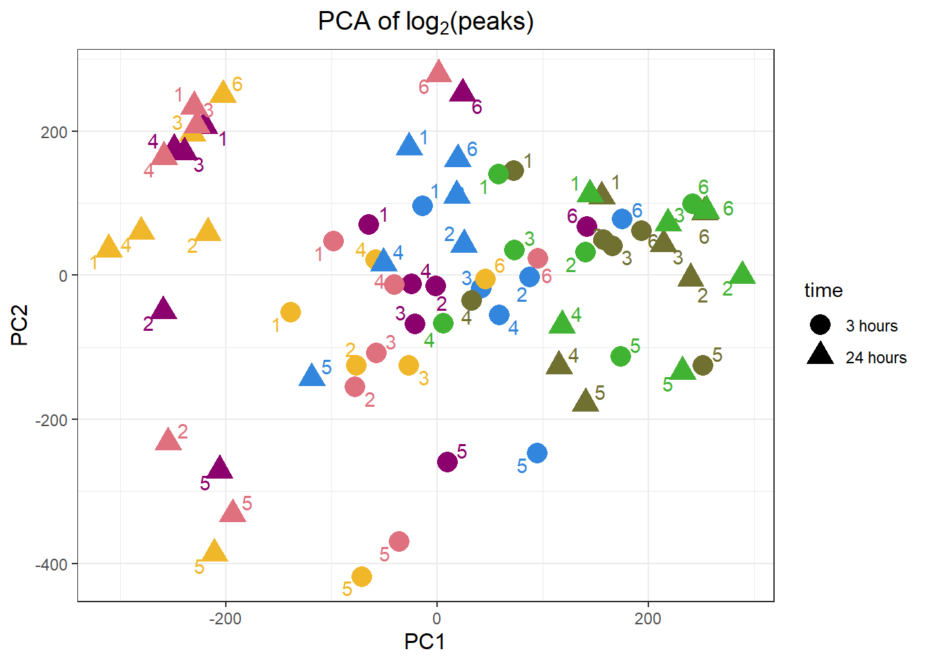
pca_all_anno %>%
  ggplot(.,aes(x = PC3, y = PC4, col=trt, shape=time, group=indv))+
  geom_point(size= 5)+
  scale_color_manual(values=drug_pal)+
   ggrepel::geom_text_repel(aes(label = indv))+
  #scale_shape_manual(name = "Time",values= c("3h"=0,"24h"=1))+
  ggtitle(expression("PCA of log"[2]*"(peaks)"))+
  theme_bw()+
  guides(col="none", size =4)+
  # labs(y = "PC 2 (15.76%)", x ="PC 1 (29.06%)")+
  theme(plot.title=element_text(size= 14,hjust = 0.5),
        axis.title = element_text(size = 12, color = "black"))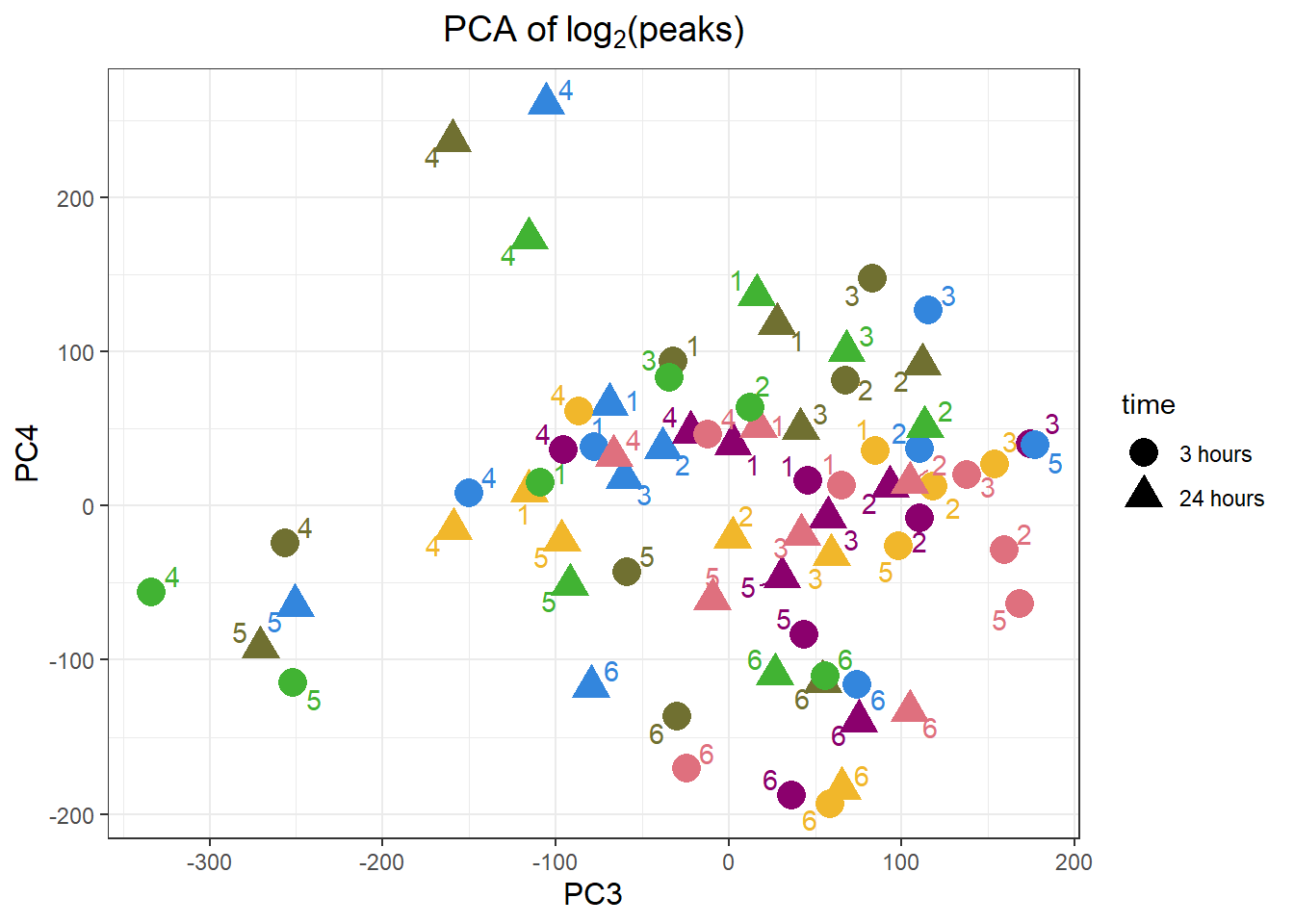
Frag_cor_filter <- filt_matrix_lcpm %>% cor()
ComplexHeatmap::pheatmap(Frag_cor_filter,
                         # column_title=(paste0("RNA-seq log"[2]~"cpm correlation")),
        annotation_col = counts_corr_mat,
        annotation_colors = mat_colors,
        heatmap_legend_param = mat_colors,
        fontsize=10,
        fontsize_row = 8,
        angle_col="90",
        treeheight_row=25,
        fontsize_col = 8,
        treeheight_col = 20)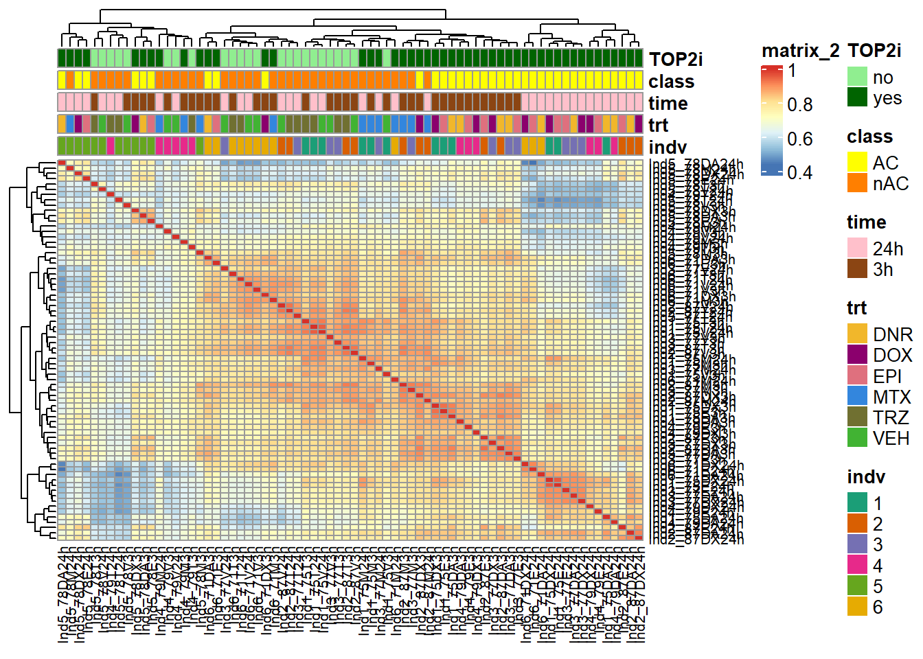
sessionInfo()R version 4.3.1 (2023-06-16 ucrt)
Platform: x86_64-w64-mingw32/x64 (64-bit)
Running under: Windows 10 x64 (build 19045)
Matrix products: default
locale:
[1] LC_COLLATE=English_United States.utf8
[2] LC_CTYPE=English_United States.utf8
[3] LC_MONETARY=English_United States.utf8
[4] LC_NUMERIC=C
[5] LC_TIME=English_United States.utf8
time zone: America/Chicago
tzcode source: internal
attached base packages:
[1] stats graphics grDevices utils datasets methods base
other attached packages:
[1] ggfortify_0.4.16 edgeR_4.0.16 limma_3.58.1 RColorBrewer_1.1-3
[5] kableExtra_1.4.0 lubridate_1.9.3 forcats_1.0.0 stringr_1.5.1
[9] dplyr_1.1.4 purrr_1.0.2 readr_2.1.5 tidyr_1.3.1
[13] tibble_3.2.1 ggplot2_3.5.0 tidyverse_2.0.0 workflowr_1.7.1
loaded via a namespace (and not attached):
[1] tidyselect_1.2.0 viridisLite_0.4.2 farver_2.1.1
[4] fastmap_1.1.1 promises_1.2.1 digest_0.6.34
[7] timechange_0.3.0 lifecycle_1.0.4 cluster_2.1.6
[10] statmod_1.5.0 processx_3.8.3 magrittr_2.0.3
[13] compiler_4.3.1 rlang_1.1.3 sass_0.4.8
[16] tools_4.3.1 utf8_1.2.4 yaml_2.3.8
[19] knitr_1.45 labeling_0.4.3 xml2_1.3.6
[22] withr_3.0.0 BiocGenerics_0.48.1 grid_4.3.1
[25] stats4_4.3.1 fansi_1.0.6 git2r_0.33.0
[28] colorspace_2.1-0 scales_1.3.0 iterators_1.0.14
[31] cli_3.6.2 rmarkdown_2.26 crayon_1.5.2
[34] generics_0.1.3 rstudioapi_0.15.0 httr_1.4.7
[37] tzdb_0.4.0 rjson_0.2.21 cachem_1.0.8
[40] parallel_4.3.1 matrixStats_1.2.0 vctrs_0.6.5
[43] jsonlite_1.8.8 callr_3.7.5 IRanges_2.36.0
[46] hms_1.1.3 GetoptLong_1.0.5 S4Vectors_0.40.2
[49] ggrepel_0.9.5 clue_0.3-65 magick_2.8.3
[52] systemfonts_1.0.5 locfit_1.5-9.9 foreach_1.5.2
[55] jquerylib_0.1.4 glue_1.7.0 codetools_0.2-19
[58] ps_1.7.6 stringi_1.8.3 gtable_0.3.4
[61] shape_1.4.6.1 later_1.3.2 ComplexHeatmap_2.18.0
[64] munsell_0.5.0 pillar_1.9.0 htmltools_0.5.7
[67] circlize_0.4.16 R6_2.5.1 doParallel_1.0.17
[70] rprojroot_2.0.4 evaluate_0.23 lattice_0.22-5
[73] highr_0.10 png_0.1-8 httpuv_1.6.14
[76] bslib_0.6.1 Rcpp_1.0.12 svglite_2.1.3
[79] gridExtra_2.3 whisker_0.4.1 xfun_0.42
[82] fs_1.6.3 getPass_0.2-4 pkgconfig_2.0.3
[85] GlobalOptions_0.1.2