TEs across histones
Renee Matthews
2026-01-30
Last updated: 2026-01-30
Checks: 7 0
Knit directory: DXR_continue/
This reproducible R Markdown analysis was created with workflowr (version 1.7.1). The Checks tab describes the reproducibility checks that were applied when the results were created. The Past versions tab lists the development history.
Great! Since the R Markdown file has been committed to the Git repository, you know the exact version of the code that produced these results.
Great job! The global environment was empty. Objects defined in the global environment can affect the analysis in your R Markdown file in unknown ways. For reproduciblity it’s best to always run the code in an empty environment.
The command set.seed(20250701) was run prior to running
the code in the R Markdown file. Setting a seed ensures that any results
that rely on randomness, e.g. subsampling or permutations, are
reproducible.
Great job! Recording the operating system, R version, and package versions is critical for reproducibility.
Nice! There were no cached chunks for this analysis, so you can be confident that you successfully produced the results during this run.
Great job! Using relative paths to the files within your workflowr project makes it easier to run your code on other machines.
Great! You are using Git for version control. Tracking code development and connecting the code version to the results is critical for reproducibility.
The results in this page were generated with repository version 5d99b72. See the Past versions tab to see a history of the changes made to the R Markdown and HTML files.
Note that you need to be careful to ensure that all relevant files for
the analysis have been committed to Git prior to generating the results
(you can use wflow_publish or
wflow_git_commit). workflowr only checks the R Markdown
file, but you know if there are other scripts or data files that it
depends on. Below is the status of the Git repository when the results
were generated:
Ignored files:
    Ignored:    .Rhistory
    Ignored:    .Rproj.user/
    Ignored:    data/Bed_exports/
    Ignored:    data/Cormotif_data/
    Ignored:    data/DER_data/
    Ignored:    data/Other_paper_data/
    Ignored:    data/RDS_files/
    Ignored:    data/TE_annotation/
    Ignored:    data/alignment_summary.txt
    Ignored:    data/all_peak_final_dataframe.txt
    Ignored:    data/cell_line_info_.tsv
    Ignored:    data/full_summary_QC_metrics.txt
    Ignored:    data/motif_lists/
    Ignored:    data/number_frag_peaks_summary.txt

Untracked files:
    Untracked:  H3K27ac_all_regions_test.bed
    Untracked:  H3K27ac_consensus_clusters_test.bed
    Untracked:  analysis/ATAC_integration_data1.Rmd
    Untracked:  analysis/GREAT_H3K27ac.Rmd
    Untracked:  analysis/H3K27ac_ChromHMM_FC.Rmd
    Untracked:  analysis/H3K27ac_TE_investigation.Rmd
    Untracked:  analysis/H3K27ac_cisRE.Rmd
    Untracked:  analysis/H3K27me3_TE_investigation.Rmd
    Untracked:  analysis/H3K36me3_TE_investigation.Rmd
    Untracked:  analysis/H3K9me3_TE_investigation.Rmd
    Untracked:  analysis/Top2a_Top2b_expression.Rmd
    Untracked:  analysis/maps_and_plots.Rmd
    Untracked:  analysis/proteomics.Rmd
    Untracked:  other_analysis/

Unstaged changes:
    Modified:   analysis/H3K27ac_RNA_integration.Rmd
    Modified:   analysis/H3K27ac_TF_motifs.Rmd
    Modified:   analysis/chromHMM.Rmd
    Modified:   analysis/final_analysis.Rmd
    Modified:   analysis/summit_files_processing.Rmd
Note that any generated files, e.g. HTML, png, CSS, etc., are not included in this status report because it is ok for generated content to have uncommitted changes.
These are the previous versions of the repository in which changes were
made to the R Markdown
(analysis/dual_histone_TE_investigation.Rmd) and HTML
(docs/dual_histone_TE_investigation.html) files. If you’ve
configured a remote Git repository (see ?wflow_git_remote),
click on the hyperlinks in the table below to view the files as they
were in that past version.
| File | Version | Author | Date | Message |
|---|---|---|---|---|
| Rmd | 5d99b72 | reneeisnowhere | 2026-01-30 | updates |
| html | 97aa671 | reneeisnowhere | 2026-01-30 | Build site. |
| Rmd | 6ec912d | reneeisnowhere | 2026-01-30 | first commits |
library(tidyverse)
library(GenomicRanges)
library(plyranges)
library(genomation)
library(readr)
library(rtracklayer)
library(stringr)
library(ggrepel)
library(DT)
library(ChIPseeker)
library(ggVennDiagram)
library(smplot2)
First steps: Pulling and overlapping each ROI set with specific families of TEs
repeatmasker <- read_delim("data/Other_paper_data/repeatmasker_20250911.txt",
    delim = "\t", escape_double = FALSE,
    trim_ws = TRUE)


autosomes <- paste0("chr", 1:22)
repeatmasker_clean <- repeatmasker %>% mutate(
    strand = ifelse(strand == "C", "-", "+")
  ) %>%
   mutate(
    start = genoStart + 1,
    end   = genoEnd)%>%
  mutate(repFamily= str_remove(repFamily, "\\?$")) %>%
  dplyr::filter(genoName %in% autosomes) %>%
  mutate(RM_id=paste0(genoName,":",start,"-",end,":",id))


rpt_split <- split(repeatmasker_clean, repeatmasker_clean$repClass)

rpt_split_gr_list <- lapply(rpt_split, function(df) {
  GRanges(
    seqnames = df$genoName,
    ranges   = IRanges(start = df$start, end = df$end),
    strand   = df$strand,
    repName   = df$repName,
    repClass  = df$repClass,
    repFamily = df$repFamily,
    swScore   = df$swScore,
    milliDiv  = df$milliDiv,
    milliDel  = df$milliDel,
    milliIns  = df$milliIns,
    RM_id        = df$RM_id
  )
})
SINE_gr <- rpt_split_gr_list$SINE
SINE_df <- SINE_gr %>%
as.data.frame()
SINE_split_df <- split(SINE_df, SINE_df$repFamily)
LINE_gr <- rpt_split_gr_list$LINE
LINE_df <- LINE_gr %>%
as.data.frame()
LINE_split_df <- split(LINE_df, LINE_df$repFamily)
LTR_gr <- rpt_split_gr_list$LTR
LTR_df <- LTR_gr %>%
as.data.frame()
LTR_split_df <- split(LTR_df, LTR_df$repFamily)
SVA_gr <- rpt_split_gr_list$Retroposon
SVA_df <- SVA_gr %>%
as.data.frame()
SVA_split_df <- split(SVA_df, SVA_df$repFamily)
DNA_gr <- rpt_split_gr_list$DNA
DNA_df <- DNA_gr %>%
as.data.frame()
DNA_split_df <- split(DNA_df, DNA_df$repFamily)Pulling in ROI granges for H3K27ac and H3K9me3
peakAnnoList_H3K9me3 <- readRDS("data/motif_lists/H3K9me3_annotated_peaks.RDS")
peakAnnoList_H3K27ac <- readRDS("data/motif_lists/H3K27ac_annotated_peaks.RDS")

H3K9me3_lookup <- imap_dfr(peakAnnoList_H3K9me3[1:3], ~
  tibble(Peakid = .x@anno$Peakid, cluster = .y)
)
H3K27ac_lookup <- imap_dfr(peakAnnoList_H3K27ac[1:3], ~
  tibble(Peakid = .x@anno$Peakid, cluster = .y)
)

H3K9me3_sets_gr <- lapply(peakAnnoList_H3K9me3, function(df) {
  as_granges(df)
})

H3K27ac_sets_gr <- lapply(peakAnnoList_H3K27ac, function(df) {
  as_granges(df)
})
H3K9me3_toplist <- readRDS( "data/DER_data/H3K9me3_toplist_nooutlier.RDS")
H3K27ac_toplist <- readRDS( "data/DER_data/H3K27ac_toplist.RDS")
H3K27ac_toptable_list <- bind_rows(H3K27ac_toplist, .id = "group")
H3K9me3_toptable_list <- bind_rows(H3K9me3_toplist, .id = "group")
K9me3_lfctable <- H3K9me3_toptable_list %>%
dplyr::select(group,genes, logFC) %>%
pivot_wider(.,id_cols = genes, names_from = group, values_from = logFC)
K27ac_lfctable <- H3K27ac_toptable_list %>%
dplyr::select(group,genes, logFC) %>%
pivot_wider(.,id_cols = genes, names_from = group, values_from = logFC)SINE
Overlapping SINE family with ROIs
sine_hits_H3K9me3 <- findOverlaps(H3K9me3_sets_gr$all_H3K9me3_regions, SINE_gr, ignore.strand = TRUE)

SINE_overlap_df_H3K9me3 <- tibble(
  peak_row = queryHits(sine_hits_H3K9me3),
  Peakid   = H3K9me3_sets_gr$all_H3K9me3$Peakid[queryHits(sine_hits_H3K9me3)],
  cluster  = H3K9me3_sets_gr$all_H3K9me3$cluster[queryHits(sine_hits_H3K9me3)],

  repClass = SINE_gr$repClass[subjectHits(sine_hits_H3K9me3)],
  repName  = SINE_gr$repName[subjectHits(sine_hits_H3K9me3)],
  RM_id  = SINE_gr$RM_id[subjectHits(sine_hits_H3K9me3)],

  TE_type  = ifelse(
    SINE_gr$repFamily[subjectHits(sine_hits_H3K9me3)] == "SVA",
    SINE_gr$repName[subjectHits(sine_hits_H3K9me3)],
    SINE_gr$repFamily[subjectHits(sine_hits_H3K9me3)]
  ),

  milliDiv = SINE_gr$milliDiv[subjectHits(sine_hits_H3K9me3)],
  milliDel = SINE_gr$milliDel[subjectHits(sine_hits_H3K9me3)],
  milliIns = SINE_gr$milliIns[subjectHits(sine_hits_H3K9me3)]
)

sine_hits_H3K27ac <- findOverlaps(H3K27ac_sets_gr$all_H3K27ac, SINE_gr, ignore.strand = TRUE)

SINE_overlap_df_H3K27ac <- tibble(
  peak_row = queryHits(sine_hits_H3K27ac),
  Peakid   = H3K27ac_sets_gr$all_H3K27ac$Peakid[queryHits(sine_hits_H3K27ac)],
  cluster  = H3K27ac_sets_gr$all_H3K27ac$cluster[queryHits(sine_hits_H3K27ac)],

  repClass = SINE_gr$repClass[subjectHits(sine_hits_H3K27ac)],
  repName  = SINE_gr$repName[subjectHits(sine_hits_H3K27ac)],
  RM_id  = SINE_gr$RM_id[subjectHits(sine_hits_H3K27ac)],

  TE_type  = ifelse(
    SINE_gr$repFamily[subjectHits(sine_hits_H3K27ac)] == "SVA",
    SINE_gr$repName[subjectHits(sine_hits_H3K27ac)],
    SINE_gr$repFamily[subjectHits(sine_hits_H3K27ac)]
  ),

  milliDiv = SINE_gr$milliDiv[subjectHits(sine_hits_H3K27ac)],
  milliDel = SINE_gr$milliDel[subjectHits(sine_hits_H3K27ac)],
  milliIns = SINE_gr$milliIns[subjectHits(sine_hits_H3K27ac)]
)

common_sine_RMs <- intersect(
  SINE_overlap_df_H3K27ac$RM_id,
  SINE_overlap_df_H3K9me3$RM_id
)

length(unique(common_sine_RMs))
[1] 7675Visualizing the overlapping SINE families
H3K27ac_SINE_peakid <- SINE_overlap_df_H3K27ac %>%
  dplyr::filter(RM_id %in% common_sine_RMs) %>%
  left_join(., H3K27ac_lookup) %>%
  distinct(Peakid)

H3K9me3_SINE_peakid <- SINE_overlap_df_H3K9me3 %>%
  dplyr::filter(RM_id %in% common_sine_RMs) %>%
  left_join(., H3K9me3_lookup) %>%
  distinct(Peakid)
I struggled with figuring out whether a TE is unique to a peak. I do have some SINE elements mapping to multiple peaks, but not a whole lot.
SINE_overlap_df_H3K9me3 %>%
  count(RM_id, name = "n_peaks") %>%
  count(n_peaks)
# A tibble: 2 × 2
n_peaks n
<int> <int>
1 1 50658
2 2 361SINE_overlap_df_H3K9me3 %>%
count(RM_id) %>%
summarise(
min = min(n),
median = median(n),
mean = mean(n),
max = max(n)
)# A tibble: 1 × 4
min median mean max
<int> <int> <dbl> <int>
1 1 1 1.01 2SINE_overlap_df_H3K27ac %>%
count(RM_id, name = "n_peaks") %>%
count(n_peaks)# A tibble: 2 × 2
n_peaks n
<int> <int>
1 1 149643
2 2 1230SINE_overlap_df_H3K27ac %>%
count(RM_id) %>%
summarise(
min = min(n),
median = median(n),
mean = mean(n),
max = max(n)
)# A tibble: 1 × 4
min median mean max
<int> <int> <dbl> <int>
1 1 1 1.01 2Because of this many to many situation, I chose to average the log fold changes of the SINE elements overlapping multiple peaks.
### linking shared RM_id to Peakid by histone ROI for LFC plotting
##

SINE_K27ac_rmid_lfc <- data_frame(RM_id=common_sine_RMs) %>%
  left_join(.,(SINE_overlap_df_H3K27ac %>%
    dplyr::filter(RM_id %in% common_sine_RMs) %>%
    distinct(RM_id,Peakid, .keep_all = TRUE) %>%
    mutate(K27ac_Peakid=Peakid) %>%
    dplyr::select(RM_id, K27ac_Peakid))) %>%
  left_join(K27ac_lfctable, by =c("K27ac_Peakid"="genes")) %>%
  group_by(RM_id) %>%
  summarize(K27ac_24T=mean(H3K27ac_24T, na.rm=TRUE),
             K27ac_24R=mean(H3K27ac_24R,na.rm=TRUE),
             K27ac_144R=mean(H3K27ac_144R, na.rm=TRUE),
            n_K27_peaks = dplyr::n(),
            .groups="drop")

SINE_K9me3_rmid_lfc <- data_frame(RM_id=common_sine_RMs) %>%
  left_join(.,(SINE_overlap_df_H3K9me3 %>%
    dplyr::filter(RM_id %in% common_sine_RMs) %>%
    distinct(RM_id,Peakid, .keep_all = TRUE) %>%
    mutate(K9me3_Peakid=Peakid) %>%
    dplyr::select(RM_id, K9me3_Peakid))) %>%
  left_join(K9me3_lfctable, by =c("K9me3_Peakid"="genes")) %>%
  group_by(RM_id) %>%
  summarize(K9me3_24T=mean(H3K9me3_24T, na.rm=TRUE),
             K9me3_24R=mean(H3K9me3_24R,na.rm=TRUE),
             K9me3_144R=mean(H3K9me3_144R, na.rm=TRUE),
            n_K27_peaks = dplyr::n(),
            .groups="drop")


SINE_RM_lfc_concordance <- tibble(RM_id = common_sine_RMs) %>%
  left_join(SINE_K27ac_rmid_lfc, by = "RM_id") %>%
  left_join(SINE_K9me3_rmid_lfc,  by = "RM_id")
Now to try to visualize this concordance. I am specifically looking at TEs that up in one and down in another.
SINE_RM_lfc_concordance %>%
  ggplot(., aes(x=K27ac_24T, y=K9me3_24T))+
  geom_point(, alpha=0.2, size=1)+
  geom_density_2d(color= "black")+
  sm_statCorr(corr_method="spearman")+
   geom_hline(yintercept = 0, linetype = "dashed", color="red") +
  geom_vline(xintercept = 0, linetype = "dashed", color="red") +
  labs(
    x = "H3K27ac logFC (24T)",
    y = "H3K9me3 logFC (24T)",
    title = "Concordance of chromatin changes at shared SINEs for 24T"
  ) +
  theme_classic()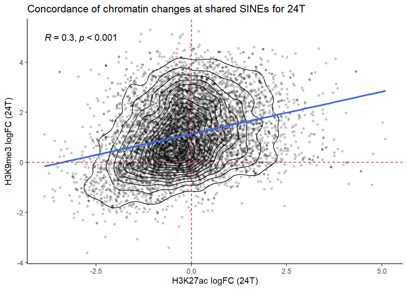
| Version | Author | Date |
|---|---|---|
| 97aa671 | reneeisnowhere | 2026-01-30 |
SINE_RM_lfc_concordance %>%
  ggplot(., aes(x=K27ac_24R, y=K9me3_24R))+
  geom_point(, alpha=0.2, size=1)+
  geom_density_2d(color= "black")+
   sm_statCorr(corr_method="spearman")+
   geom_hline(yintercept = 0, linetype = "dashed", color="red") +
  geom_vline(xintercept = 0, linetype = "dashed", color="red") +
  labs(
    x = "H3K27ac logFC (24R)",
    y = "H3K9me3 logFC (24R)",
    title = "Concordance of chromatin changes at shared SINEs for 24R"
  ) +
  theme_classic()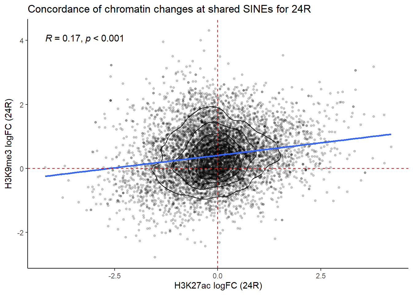
| Version | Author | Date |
|---|---|---|
| 97aa671 | reneeisnowhere | 2026-01-30 |
SINE_RM_lfc_concordance %>%
  ggplot(., aes(x=K27ac_144R, y=K9me3_144R))+
  geom_point(, alpha=0.2, size=1)+
  geom_density_2d(color= "black")+
   sm_statCorr(corr_method="spearman")+
   geom_hline(yintercept = 0, linetype = "dashed", color="red") +
  geom_vline(xintercept = 0, linetype = "dashed", color="red") +
  labs(
    x = "H3K27ac logFC (144R)",
    y = "H3K9me3 logFC (144R)",
    title = "Concordance of chromatin changes at shared SINEs for 144R"
  ) +
  theme_classic()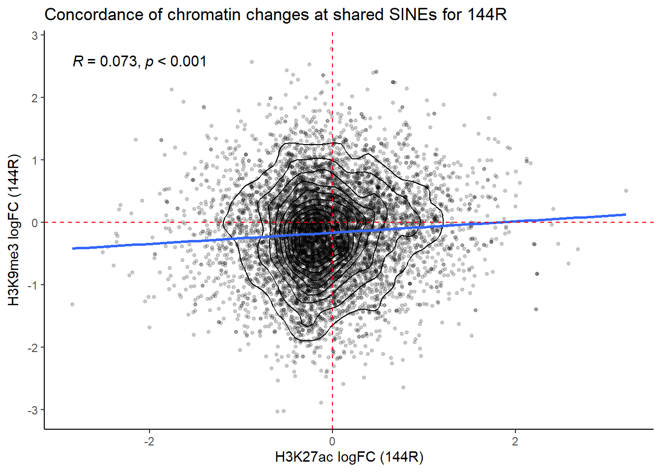
| Version | Author | Date |
|---|---|---|
| 97aa671 | reneeisnowhere | 2026-01-30 |
LTR
Overlapping LTR family with ROIs
LTR_hits_H3K9me3 <- findOverlaps(H3K9me3_sets_gr$all_H3K9me3_regions, LTR_gr, ignore.strand = TRUE)

LTR_overlap_df_H3K9me3 <- tibble(
  peak_row = queryHits(LTR_hits_H3K9me3),
  Peakid   = H3K9me3_sets_gr$all_H3K9me3$Peakid[queryHits(LTR_hits_H3K9me3)],
  cluster  = H3K9me3_sets_gr$all_H3K9me3$cluster[queryHits(LTR_hits_H3K9me3)],

  repClass = LTR_gr$repClass[subjectHits(LTR_hits_H3K9me3)],
  repName  = LTR_gr$repName[subjectHits(LTR_hits_H3K9me3)],
  RM_id  = LTR_gr$RM_id[subjectHits(LTR_hits_H3K9me3)],

  TE_type  = ifelse(
    LTR_gr$repFamily[subjectHits(LTR_hits_H3K9me3)] == "SVA",
    LTR_gr$repName[subjectHits(LTR_hits_H3K9me3)],
    LTR_gr$repFamily[subjectHits(LTR_hits_H3K9me3)]
  ),

  milliDiv = LTR_gr$milliDiv[subjectHits(LTR_hits_H3K9me3)],
  milliDel = LTR_gr$milliDel[subjectHits(LTR_hits_H3K9me3)],
  milliIns = LTR_gr$milliIns[subjectHits(LTR_hits_H3K9me3)]
)

LTR_hits_H3K27ac <- findOverlaps(H3K27ac_sets_gr$all_H3K27ac, LTR_gr, ignore.strand = TRUE)

LTR_overlap_df_H3K27ac <- tibble(
  peak_row = queryHits(LTR_hits_H3K27ac),
  Peakid   = H3K27ac_sets_gr$all_H3K27ac$Peakid[queryHits(LTR_hits_H3K27ac)],
  cluster  = H3K27ac_sets_gr$all_H3K27ac$cluster[queryHits(LTR_hits_H3K27ac)],

  repClass = LTR_gr$repClass[subjectHits(LTR_hits_H3K27ac)],
  repName  = LTR_gr$repName[subjectHits(LTR_hits_H3K27ac)],
  RM_id  = LTR_gr$RM_id[subjectHits(LTR_hits_H3K27ac)],

  TE_type  = ifelse(
    LTR_gr$repFamily[subjectHits(LTR_hits_H3K27ac)] == "SVA",
    LTR_gr$repName[subjectHits(LTR_hits_H3K27ac)],
    LTR_gr$repFamily[subjectHits(LTR_hits_H3K27ac)]
  ),

  milliDiv = LTR_gr$milliDiv[subjectHits(LTR_hits_H3K27ac)],
  milliDel = LTR_gr$milliDel[subjectHits(LTR_hits_H3K27ac)],
  milliIns = LTR_gr$milliIns[subjectHits(LTR_hits_H3K27ac)]
)

common_LTR_RMs <- intersect(
  LTR_overlap_df_H3K27ac$RM_id,
  LTR_overlap_df_H3K9me3$RM_id
)

length(unique(common_LTR_RMs))
[1] 5947Visualizing the overlapping LTR families
H3K27ac_LTR_peakid <- LTR_overlap_df_H3K27ac %>%
  dplyr::filter(RM_id %in% common_LTR_RMs) %>%
  left_join(., H3K27ac_lookup) %>%
  distinct(Peakid)

H3K9me3_LTR_peakid <- LTR_overlap_df_H3K9me3 %>%
  dplyr::filter(RM_id %in% common_LTR_RMs) %>%
  left_join(., H3K9me3_lookup) %>%
  distinct(Peakid)
I struggled with figuring out whether a TE is unique to a peak. I do have some LTR elements mapping to multiple peaks, and more than SINEs most likely due to the increased TE lengths.
LTR_overlap_df_H3K9me3 %>%
  count(RM_id, name = "n_peaks") %>%
  count(n_peaks)
# A tibble: 8 × 2
n_peaks n
<int> <int>
1 1 74479
2 2 4627
3 3 458
4 4 133
5 5 35
6 6 21
7 7 3
8 8 2LTR_overlap_df_H3K9me3 %>%
count(RM_id) %>%
summarise(
min = min(n),
median = median(n),
mean = mean(n),
max = max(n)
)# A tibble: 1 × 4
min median mean max
<int> <dbl> <dbl> <int>
1 1 1 1.08 8LTR_overlap_df_H3K27ac %>%
count(RM_id, name = "n_peaks") %>%
count(n_peaks)# A tibble: 4 × 2
n_peaks n
<int> <int>
1 1 35045
2 2 421
3 3 13
4 4 4LTR_overlap_df_H3K27ac %>%
count(RM_id) %>%
summarise(
min = min(n),
median = median(n),
mean = mean(n),
max = max(n)
)# A tibble: 1 × 4
min median mean max
<int> <int> <dbl> <int>
1 1 1 1.01 4Because of this many to many situation, I chose to average the log fold changes of the LTR elements overlapping multiple peaks.
### linking shared RM_id to Peakid by histone ROI for LFC plotting
##

K27ac_rmid_lfc <- data_frame(RM_id=common_LTR_RMs) %>%
  left_join(.,(LTR_overlap_df_H3K27ac %>%
    dplyr::filter(RM_id %in% common_LTR_RMs) %>%
    distinct(RM_id,Peakid, .keep_all = TRUE))) %>%
    mutate(K27ac_Peakid=Peakid) %>%
    dplyr::select(RM_id, K27ac_Peakid) %>%
  left_join(K27ac_lfctable, by =c("K27ac_Peakid"="genes")) %>%
  left_join(., H3K27ac_lookup, by =c("K27ac_Peakid"="Peakid")) %>%
  group_by(RM_id) %>%
  summarize(K27ac_24T=mean(H3K27ac_24T, na.rm=TRUE),
             K27ac_24R=mean(H3K27ac_24R,na.rm=TRUE),
             K27ac_144R=mean(H3K27ac_144R, na.rm=TRUE),
            n_K27ac_peaks = dplyr::n(),
            cluster=dplyr::first(cluster),
            .groups="drop") %>%
   tidyr::replace_na(list(cluster = "NA"))

K9me3_rmid_lfc <- data_frame(RM_id=common_LTR_RMs) %>%
  left_join(.,(LTR_overlap_df_H3K9me3 %>%
    dplyr::filter(RM_id %in% common_LTR_RMs) %>%
    distinct(RM_id,Peakid, .keep_all = TRUE) %>%
    mutate(K9me3_Peakid=Peakid) %>%
    dplyr::select(RM_id, K9me3_Peakid))) %>%
  left_join(K9me3_lfctable, by =c("K9me3_Peakid"="genes")) %>%
  group_by(RM_id) %>%
  summarize(K9me3_24T=mean(H3K9me3_24T, na.rm=TRUE),
             K9me3_24R=mean(H3K9me3_24R,na.rm=TRUE),
             K9me3_144R=mean(H3K9me3_144R, na.rm=TRUE),
            n_K9me3_peaks = dplyr::n(),
            .groups="drop")


LTR_RM_lfc_concordance <- tibble(RM_id = common_LTR_RMs) %>%
  left_join(K27ac_rmid_lfc, by = "RM_id") %>%
  left_join(K9me3_rmid_lfc,  by = "RM_id")
Now to try to visualize this concordance. I am specifically looking at TEs that up in one and down in another.
LTR_RM_lfc_concordance %>%
  ggplot(., aes(x=K27ac_24T, y=K9me3_24T, color=cluster))+
  geom_point(, alpha=0.2, size=2)+
  geom_density_2d(color= "black")+
   # sm_statCorr(corr_method="spearman")+
   geom_hline(yintercept = 0, linetype = "dashed", color="red") +
  geom_vline(xintercept = 0, linetype = "dashed", color="red") +
  labs(
    x = "H3K27ac logFC (24T)",
    y = "H3K9me3 logFC (24T)",
    title = "Concordance of chromatin changes at shared LTRs for 24T"
  ) +
  theme_classic()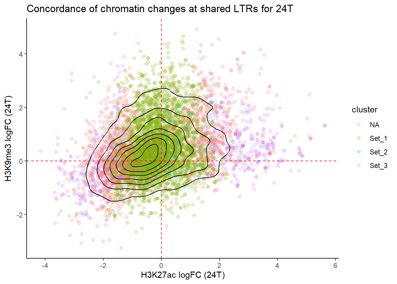
| Version | Author | Date |
|---|---|---|
| 97aa671 | reneeisnowhere | 2026-01-30 |
LTR_RM_lfc_concordance %>%
  ggplot(., aes(x=K27ac_24R, y=K9me3_24R, color=cluster))+
  geom_point(, alpha=0.2, size=2)+
  geom_density_2d(color= "black")+
   # sm_statCorr(corr_method="spearman")+
   geom_hline(yintercept = 0, linetype = "dashed", color="red") +
  geom_vline(xintercept = 0, linetype = "dashed", color="red") +
  labs(
    x = "H3K27ac logFC (24R)",
    y = "H3K9me3 logFC (24R)",
    title = "Concordance of chromatin changes at shared LTRs for 24R"
  ) +
  theme_classic()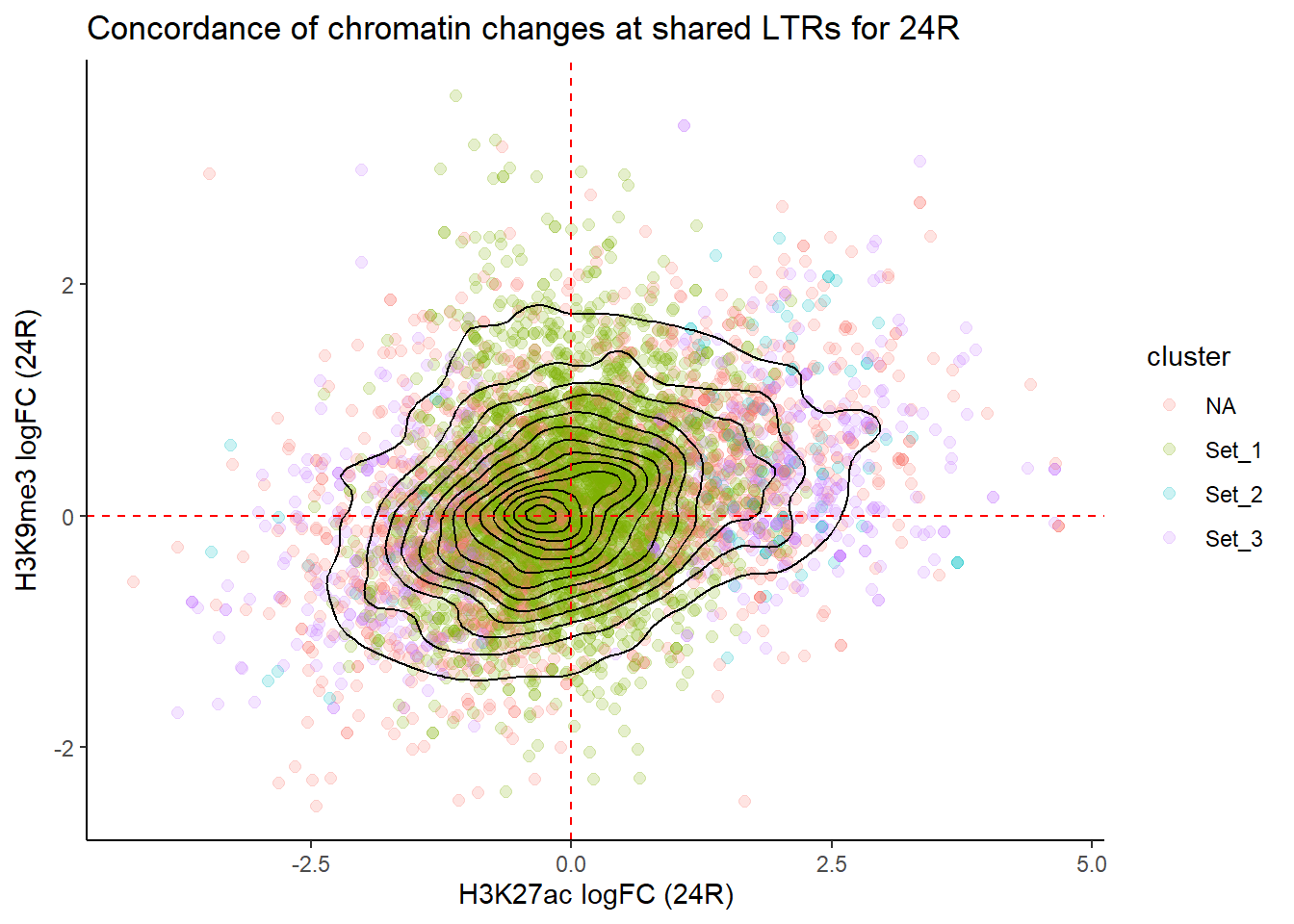
| Version | Author | Date |
|---|---|---|
| 97aa671 | reneeisnowhere | 2026-01-30 |
LTR_RM_lfc_concordance %>%
  ggplot(., aes(x=K27ac_144R, y=K9me3_144R, color=cluster))+
  geom_point(, alpha=0.2, size=2)+
  geom_density_2d(color= "black")+
     # sm_statCorr(corr_method="spearman")+

   geom_hline(yintercept = 0, linetype = "dashed", color="red") +
  geom_vline(xintercept = 0, linetype = "dashed", color="red") +
  labs(
    x = "H3K27ac logFC (144R)",
    y = "H3K9me3 logFC (144R)",
    title = "Concordance of chromatin changes at shared LTRs for 144R"
  ) +
  theme_classic()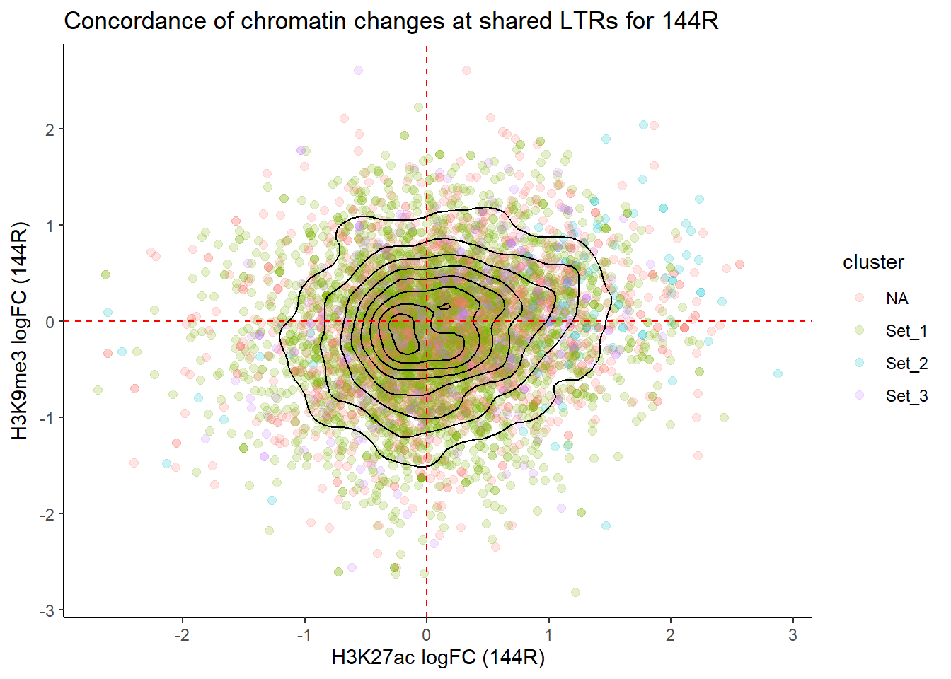
| Version | Author | Date |
|---|---|---|
| 97aa671 | reneeisnowhere | 2026-01-30 |
LTR_RM_lfc_concordance %>%
  ggplot(., aes(x=K27ac_24T, y=K27ac_24R, color=cluster))+
  geom_point(, alpha=0.2, size=2)+
  geom_density_2d(color= "black")+
   # sm_statCorr(corr_method="spearman")+
   geom_hline(yintercept = 0, linetype = "dashed", color="red") +
  geom_vline(xintercept = 0, linetype = "dashed", color="red") +
  labs(
    x = "H3K27ac logFC (24T)",
    y = "H3K9me3 logFC (24T)",
    title = "Concordance of chromatin changes at shared LTRs for 24T v 24R H3K27ac"
  ) +
  theme_classic()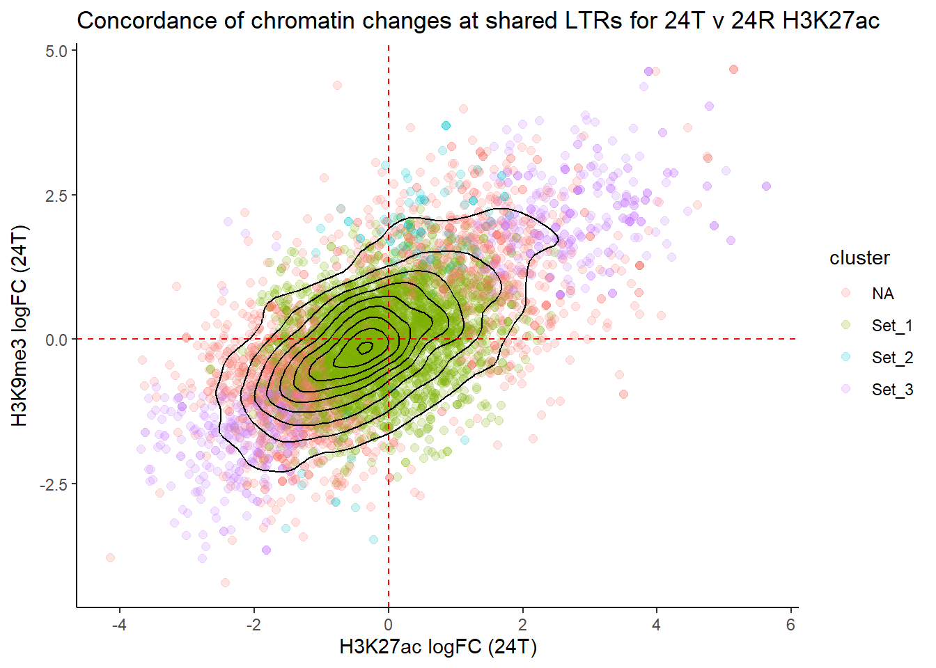
LTR_RM_lfc_concordance %>%
  ggplot(., aes(x=K27ac_24T, y=K27ac_144R, color=cluster))+
  geom_point(, alpha=0.2, size=2)+
  geom_density_2d(color= "black")+
   # sm_statCorr(corr_method="spearman")+
   geom_hline(yintercept = 0, linetype = "dashed", color="red") +
  geom_vline(xintercept = 0, linetype = "dashed", color="red") +
  labs(
    x = "H3K27ac logFC (24T)",
    y = "H3K9me3 logFC (24T)",
    title = "Concordance of chromatin changes at shared LTRs for 24T v 144R H3K27ac"
  ) +
  theme_classic()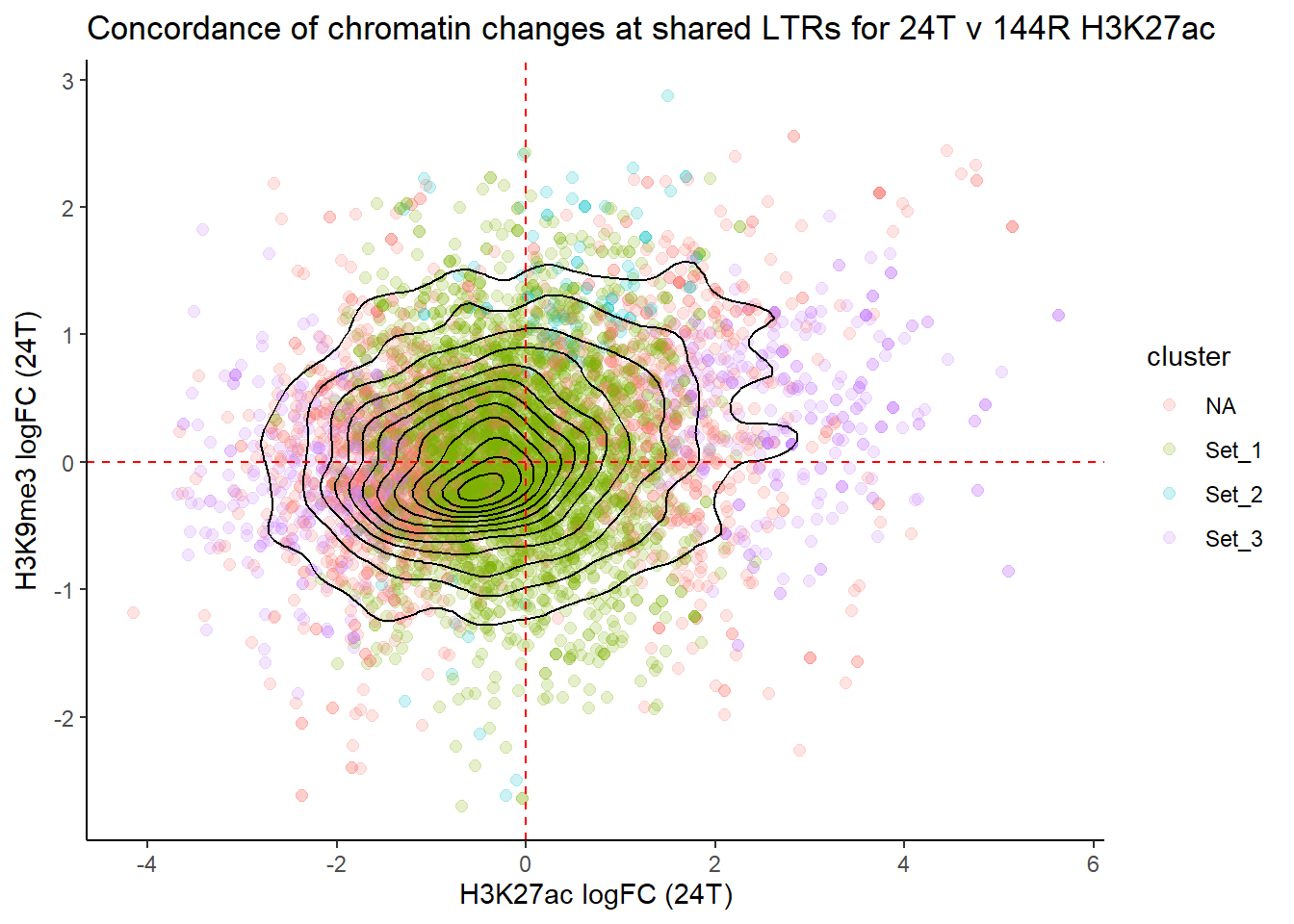
LTR_RM_lfc_concordance %>%
  ggplot(., aes(x=K27ac_24R, y=K27ac_144R, color=cluster))+
  geom_point(, alpha=0.2, size=2)+
  geom_density_2d(color= "black")+
   # sm_statCorr(corr_method="spearman")+
   geom_hline(yintercept = 0, linetype = "dashed", color="red") +
  geom_vline(xintercept = 0, linetype = "dashed", color="red") +
  labs(
    x = "H3K27ac logFC (24T)",
    y = "H3K9me3 logFC (24T)",
    title = "Concordance of chromatin changes at shared LTRs for 24R v 144R H3K27ac"
  ) +
  theme_classic()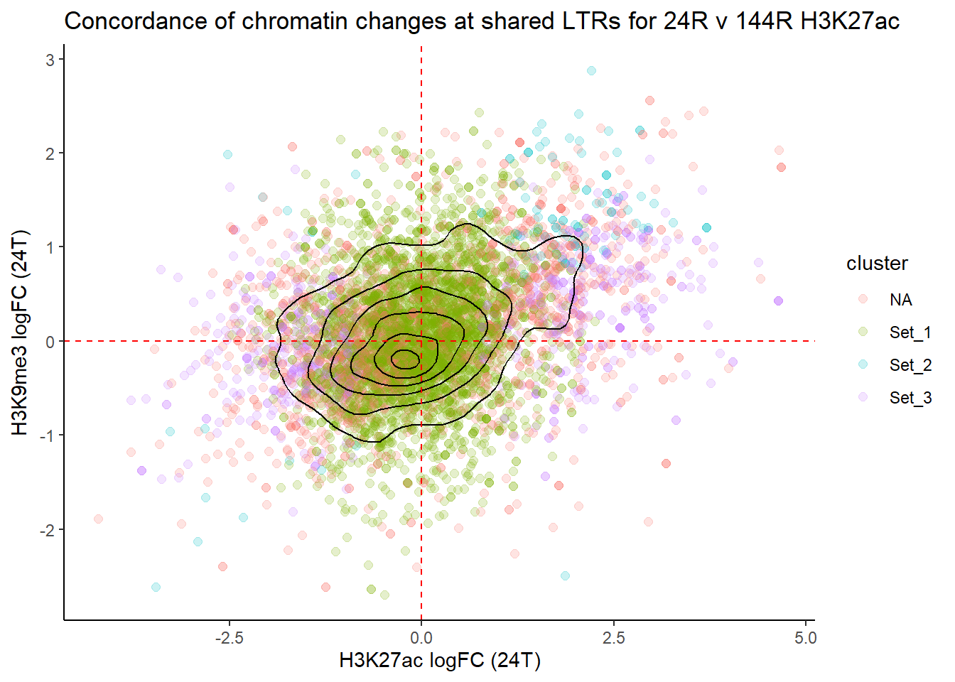
K27ac_unfiltered_long <- K27ac_lfctable %>%
  left_join(H3K27ac_lookup, by = c("genes" = "Peakid")) %>%
  tidyr::replace_na(list(cluster = "NA")) %>%
  dplyr::filter(cluster != "NA") %>%
  pivot_longer(
    cols = c("H3K27ac_24T", "H3K27ac_24R", "H3K27ac_144R"),
    names_to = "group",
    values_to = "LFC") %>%
  mutate(group = factor(group, levels = c("H3K27ac_24T", "H3K27ac_24R", "H3K27ac_144R")))

K9me3_unfiltered_long <- K9me3_lfctable %>%
  left_join(H3K9me3_lookup, by = c("genes" = "Peakid")) %>%
  tidyr::replace_na(list(cluster = "NA")) %>%
  dplyr::filter(cluster != "NA") %>%
  pivot_longer(
    cols = c("H3K9me3_24T", "H3K9me3_24R", "H3K9me3_144R"),
    names_to = "group",
    values_to = "LFC") %>%
  mutate(group = factor(group, levels = c("H3K9me3_24T", "H3K9me3_24R", "H3K9me3_144R")))

K27ac_median_unfilt_lfc <- K27ac_unfiltered_long %>%
  group_by(cluster, group) %>%
  summarise(median_abs_LFC = median(abs(LFC), na.rm = TRUE),
            .groups = "drop")%>%
  mutate(time=str_remove(group,"H3K27ac"))%>%
  mutate(time=factor(time, levels=c("_24T","_24R","_144R")))

K9me3_median_unfilt_lfc <- K9me3_unfiltered_long %>%
  group_by(cluster, group) %>%
  summarise(median_abs_LFC = median(abs(LFC), na.rm = TRUE),
            .groups = "drop")%>%
  mutate(time=str_remove(group,"H3K9me3")) %>%
  mutate(time=factor(time, levels=c("_24T","_24R","_144R")))

K9me3_median_unfilt_lfc %>%
  ggplot(., aes(x=group, y=median_abs_LFC, group=cluster, color=cluster))+
  geom_point(size=4)+
  geom_line(aes(alpha = 0.8, linewidth = 4))+
  theme_bw()+
  ggtitle("LFC across time for H3K27ac sets")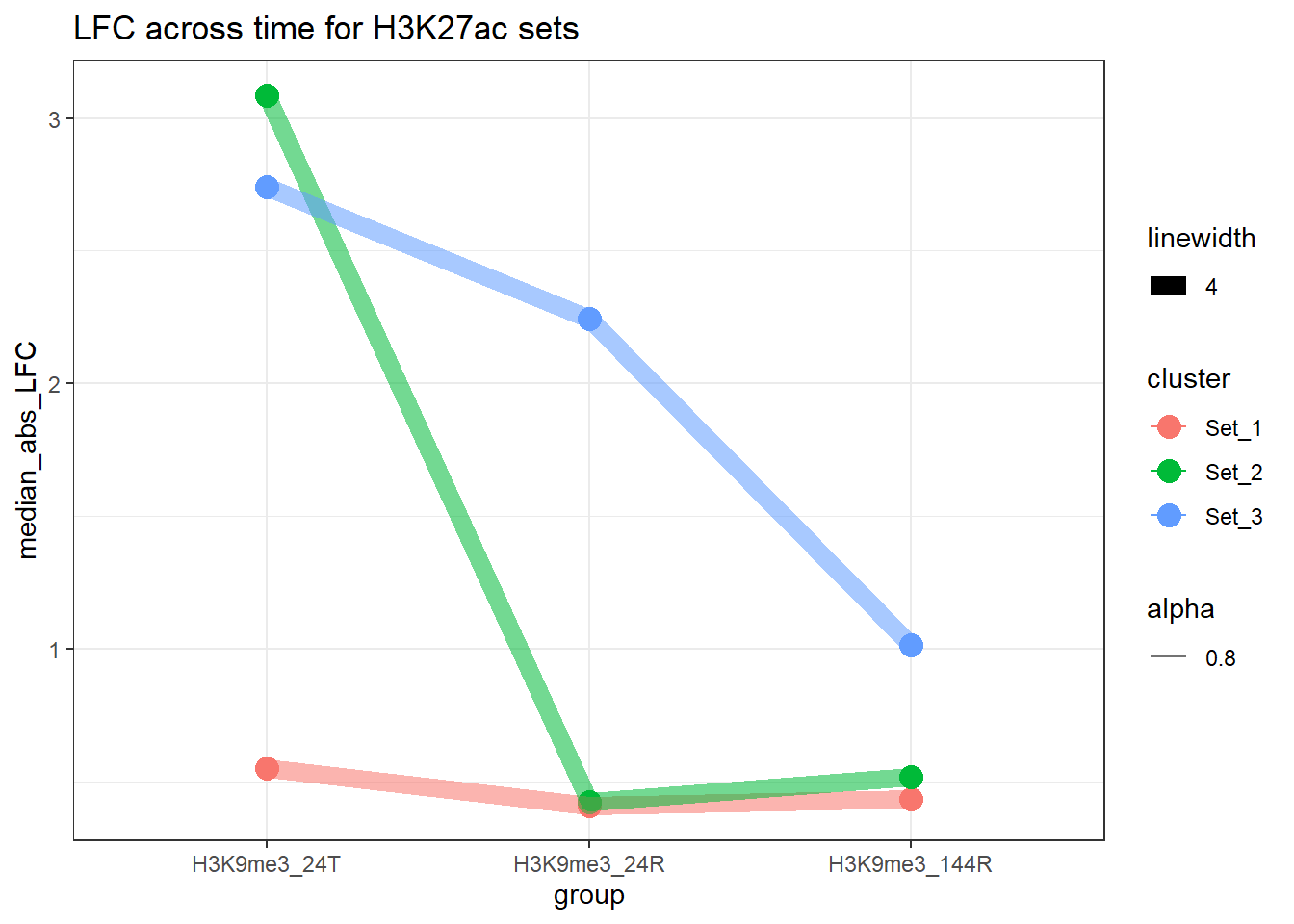
| Version | Author | Date |
|---|---|---|
| 97aa671 | reneeisnowhere | 2026-01-30 |
K27ac_median_LTR_lfc <- K27ac_unfiltered_long %>%
  dplyr::filter(genes %in% H3K27ac_LTR_peakid$Peakid) %>%
  group_by(cluster, group) %>%
  summarise(median_abs_LFC = median(abs(LFC), na.rm = TRUE),
            .groups = "drop") %>%
  mutate(time=str_remove(group,"H3K27ac"))%>%
  mutate(time=factor(time, levels=c("_24T","_24R","_144R")))
K9me3_median_LTR_lfc <- K9me3_unfiltered_long %>%
  dplyr::filter(genes %in% H3K9me3_LTR_peakid$Peakid) %>%
  group_by(cluster, group) %>%
  summarise(median_abs_LFC = median(abs(LFC), na.rm = TRUE),
            .groups = "drop") %>%
  mutate(time=str_remove(group,"H3K9me3"))%>%
  mutate(time=factor(time, levels=c("_24T","_24R","_144R")))

K9me3_median_unfilt_lfc %>%
ggplot(., aes(x=time, y=median_abs_LFC, group=cluster, color=cluster))+
  geom_point(size=4)+
  geom_line(aes(alpha = 0.8, linewidth = 4))+

  geom_line(data=K27ac_median_unfilt_lfc, aes(x=time,y=median_abs_LFC, group=cluster,color=cluster), linetype=2, size = 1)+
   geom_point(data=K27ac_median_unfilt_lfc, aes(x=time,y=median_abs_LFC, group=cluster,color=cluster), linetype=2, size = 1)+
  theme_bw()+
  ggtitle("H3K9me3 unfiltered solid line\nH3K27ac dotted line absolute LFC All regions")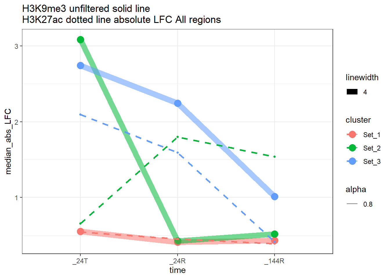
| Version | Author | Date |
|---|---|---|
| 97aa671 | reneeisnowhere | 2026-01-30 |
K9me3_median_LTR_lfc %>%
ggplot(., aes(x=time, y=median_abs_LFC, group=cluster, color=cluster))+
  geom_point(size=4)+
  geom_line(aes(alpha = 0.8, linewidth = 4))+

  geom_line(data=K27ac_median_LTR_lfc, aes(x=time,y=median_abs_LFC, group=cluster,color=cluster), linetype=2, size = 1)+
   geom_point(data=K27ac_median_LTR_lfc, aes(x=time,y=median_abs_LFC, group=cluster,color=cluster), linetype=2, size = 1)+
  theme_bw()+
  ggtitle("H3K9me3 solid line\nH3K27ac dotted line absolute LFC overlapping LTR regions")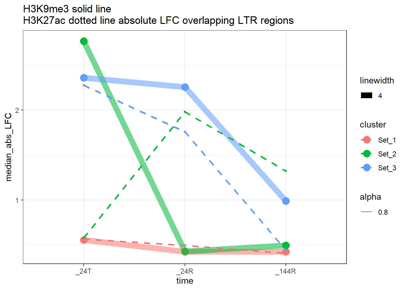
| Version | Author | Date |
|---|---|---|
| 97aa671 | reneeisnowhere | 2026-01-30 |
Now I am trying to break down by LTR families:
LTR_overlap_df_H3K27ac %>%
  group_by(TE_type) %>%
  tally() %>%
   ungroup() %>%
  DT::datatable(
    rownames = FALSE,
    caption = htmltools::tags$caption(
      style = "caption-side: top; text-align: left;",
      "H3K27ac LTR specific overlap counts by TE familiy"),
    options = list(pageLength = 10,
      autoWidth = TRUE,
      dom = "tip"))
# now I want to breakup common_LTR_RMs and plot by family of LTR.
K27_family_plot <- function(lfc_df,
split_list,
grp="K27ac",
repFamily,
repName){
rm_ids <- split_list[[repName]]$RM_id
lfc_df %>%
dplyr::filter(RM_id %in% rm_ids) %>%
dplyr::filter(cluster != "NA") %>%
pivot_longer(.,cols=c(starts_with(grp)), names_to="group", values_to = "LFC") %>%
group_by(cluster, group) %>%
summarise(median_abs_LFC = median(abs(LFC), na.rm = TRUE),
.groups = "drop")%>%
mutate(time=str_remove(group,grp))%>%
mutate(time=factor(time, levels=c("_24T","_24R","_144R"))) %>%
ggplot(., aes(x=time, y=median_abs_LFC, group=cluster, color=cluster))+
geom_point(size=4)+
geom_line(aes(alpha = 0.8, linewidth = 4))+
theme_bw()+
ggtitle(paste0(grp," absolute LFC overlapping ",repFamily,":",repName))
}names(LTR_split_df)[1] "ERV1" "ERVK" "ERVL" "ERVL-MaLR" "Gypsy" "LTR" K27_family_plot(K27ac_rmid_lfc, LTR_split_df,"K27ac","LTR","ERV1")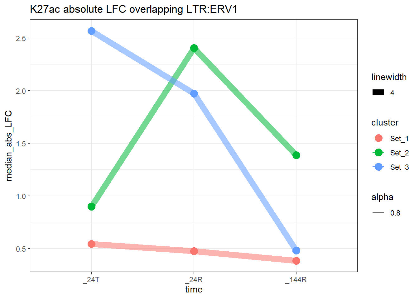
K27_family_plot(K27ac_rmid_lfc, LTR_split_df,"K27ac","LTR","ERVK")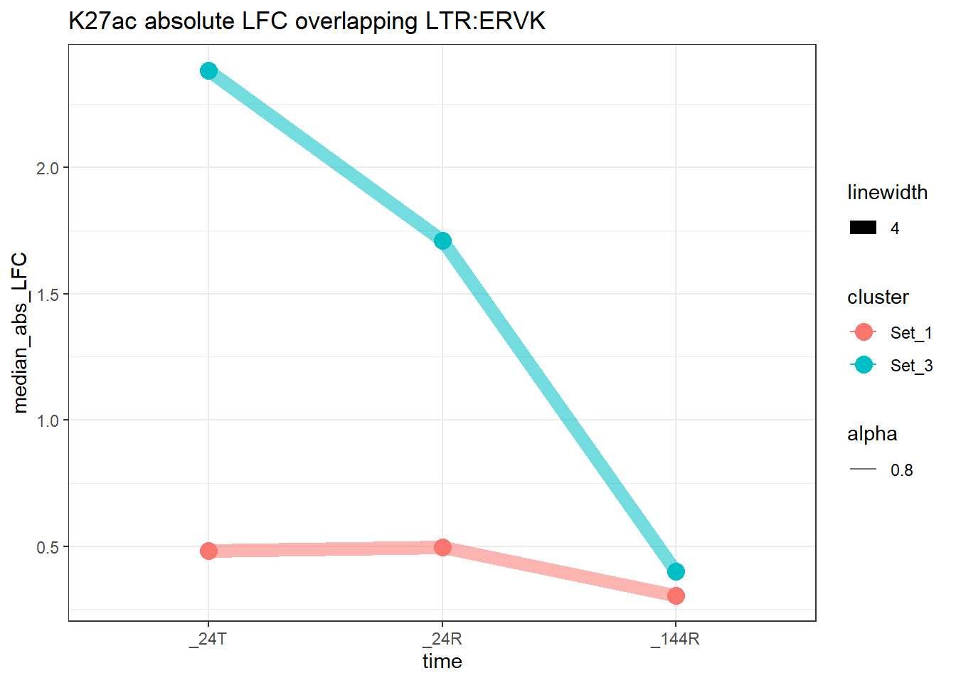
K27_family_plot(K27ac_rmid_lfc, LTR_split_df,"K27ac","LTR","ERVL")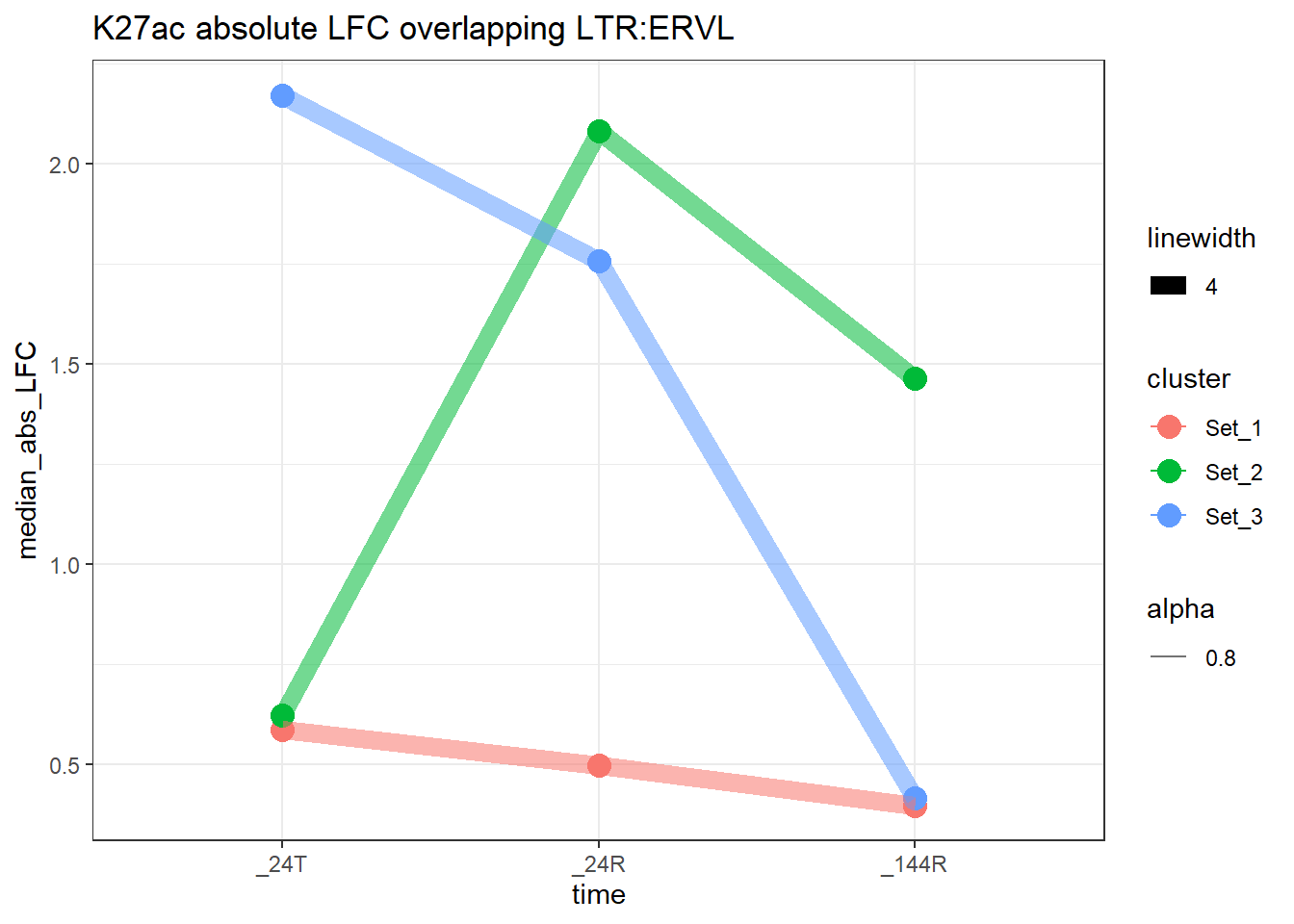
K27_family_plot(K27ac_rmid_lfc, LTR_split_df,"K27ac","LTR","ERVL-MaLR")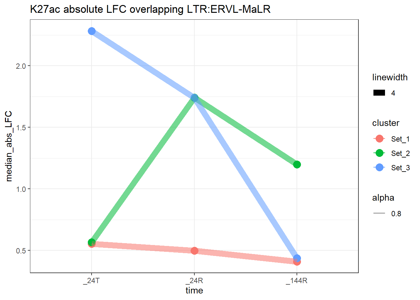
K27_family_plot(K27ac_rmid_lfc, LTR_split_df,"K27ac","LTR","Gypsy")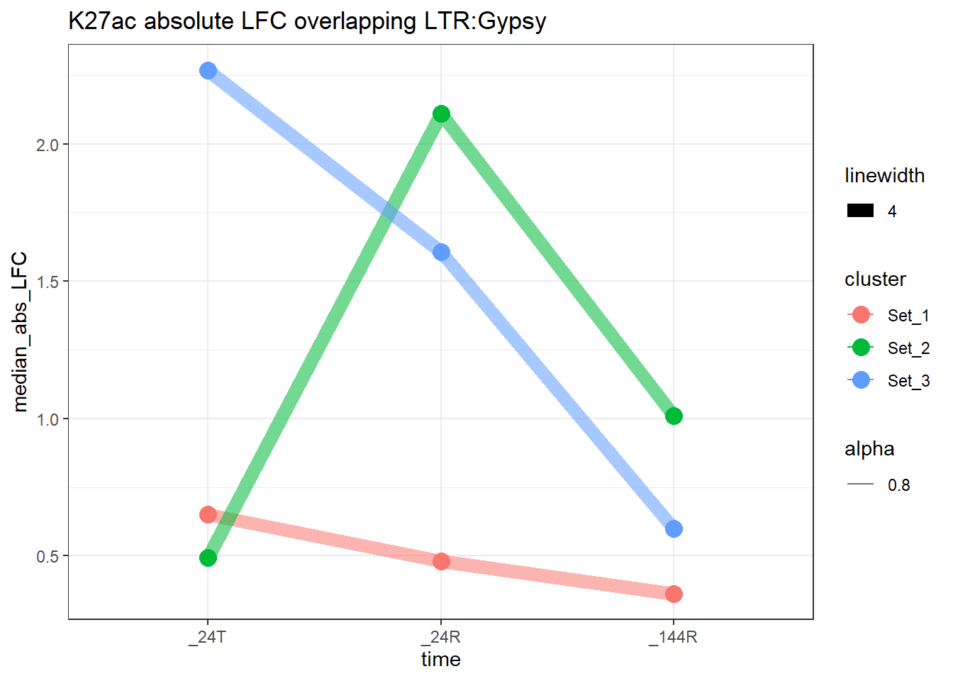
K27_family_plot(K27ac_rmid_lfc, LTR_split_df,"K27ac","LTR","LTR")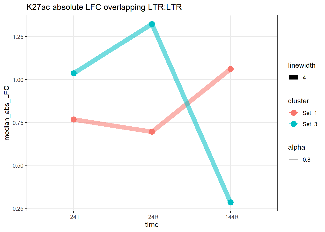
K27_K9_family_plot <- function(lfc_df,
                            split_list,
                            marks=c("K27ac","K9me3"),
                            repClass,
                            repFam){


  rm_ids <- split_list[[repFam]]$RM_id

  lfc_df %>%
  dplyr::filter(RM_id %in% rm_ids,
                cluster != "NA") %>%
  pivot_longer(.,cols=tidyselect::matches(paste0("^(",paste(marks,collapse = "|"), ")")),
               names_to="group",
               values_to = "LFC") %>%
     mutate(mark = stringr::str_extract(group, paste(marks, collapse="|")),
      time = stringr::str_remove(group, paste(marks, collapse="|")),
      time = factor(time, levels = c("_24T", "_24R", "_144R"))) %>%
  group_by(cluster, mark ,time) %>%
  summarise(median_abs_LFC = median(abs(LFC), na.rm = TRUE),
            .groups = "drop")%>%
  ggplot(., aes(x=time, y=median_abs_LFC, group=interaction(cluster,mark), color=cluster, linetype=mark, shape=mark))+
  geom_point(size=4)+
  geom_line(aes(alpha = 0.8, linewidth = 4))+
  theme_bw()+
  labs(title = paste0("Both histones, absolute LFC overlapping ",repClass,":",repFam),
      y = "Median |LFC|",
      x = "Time"
    )
}
K27_K9_family_plot(LTR_RM_lfc_concordance, LTR_split_df,marks=c("K27ac","K9me3"), "LTR",repFam="ERVL")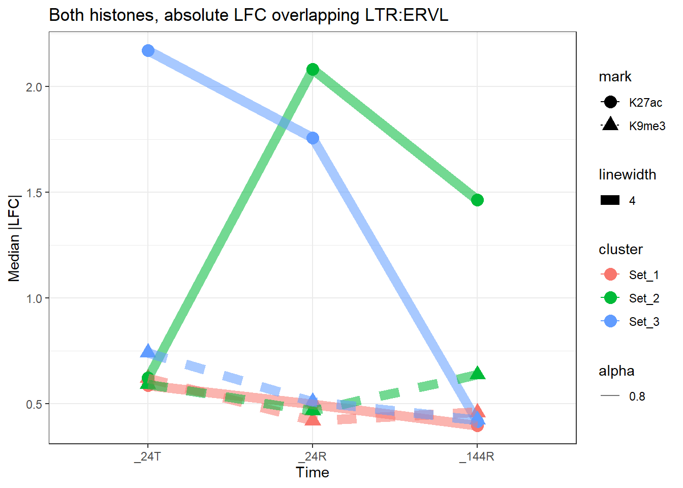
K27_K9_family_plot(LTR_RM_lfc_concordance, LTR_split_df,marks=c("K27ac","K9me3"), "LTR",repFam="ERVK")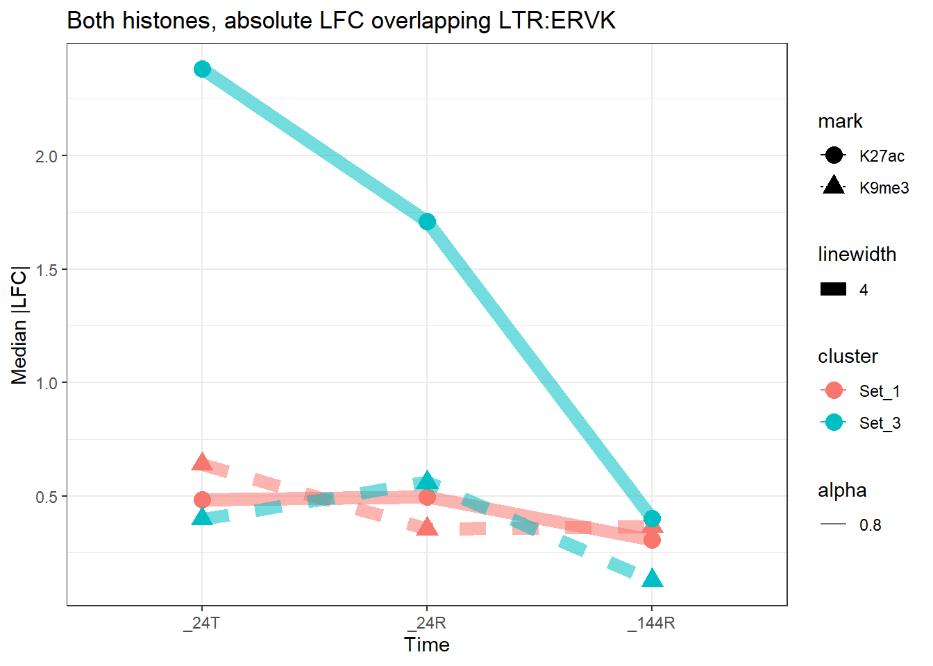
K27_K9_family_plot(LTR_RM_lfc_concordance, LTR_split_df,marks=c("K27ac","K9me3"), "LTR",repFam="ERV1")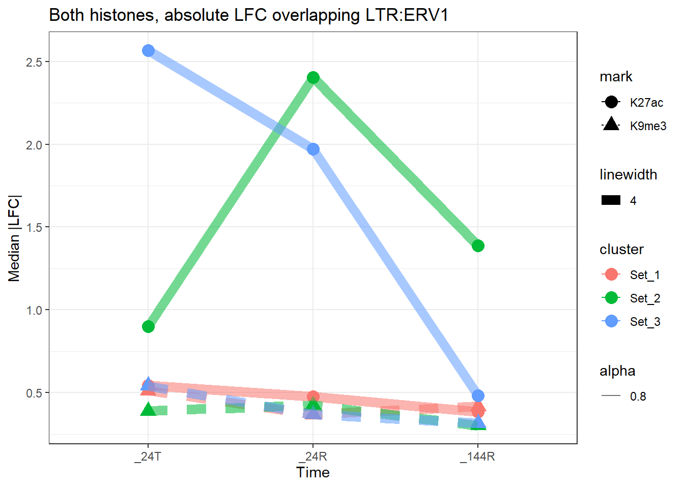
K27_K9_family_plot(LTR_RM_lfc_concordance, LTR_split_df,marks=c("K27ac","K9me3"), "LTR",repFam="ERVL-MaLR")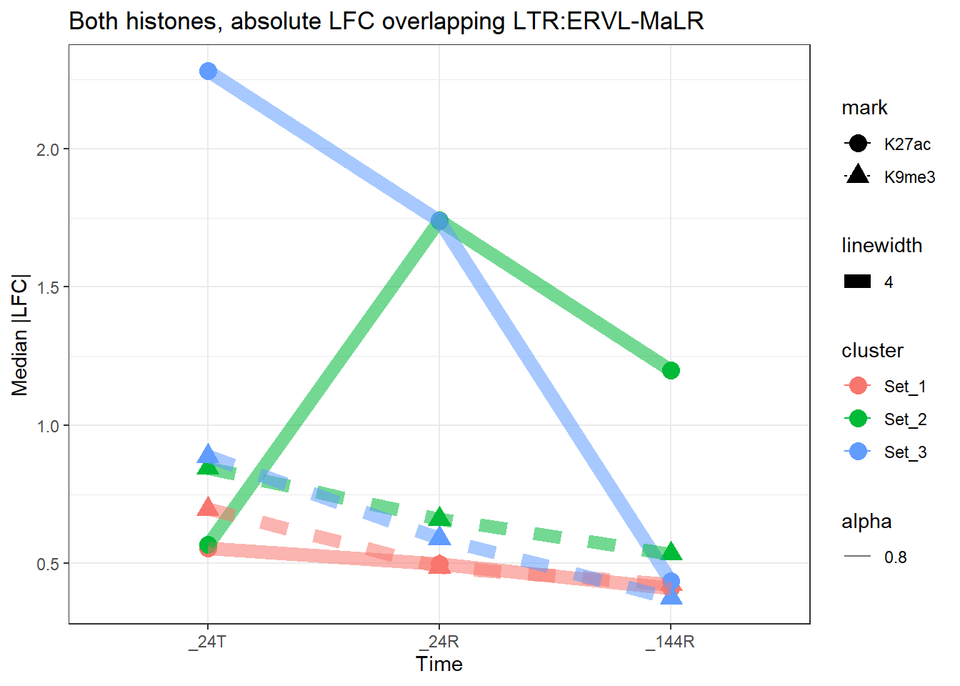
K27_K9_family_plot(LTR_RM_lfc_concordance, LTR_split_df,marks=c("K27ac","K9me3"), "LTR",repFam="Gypsy")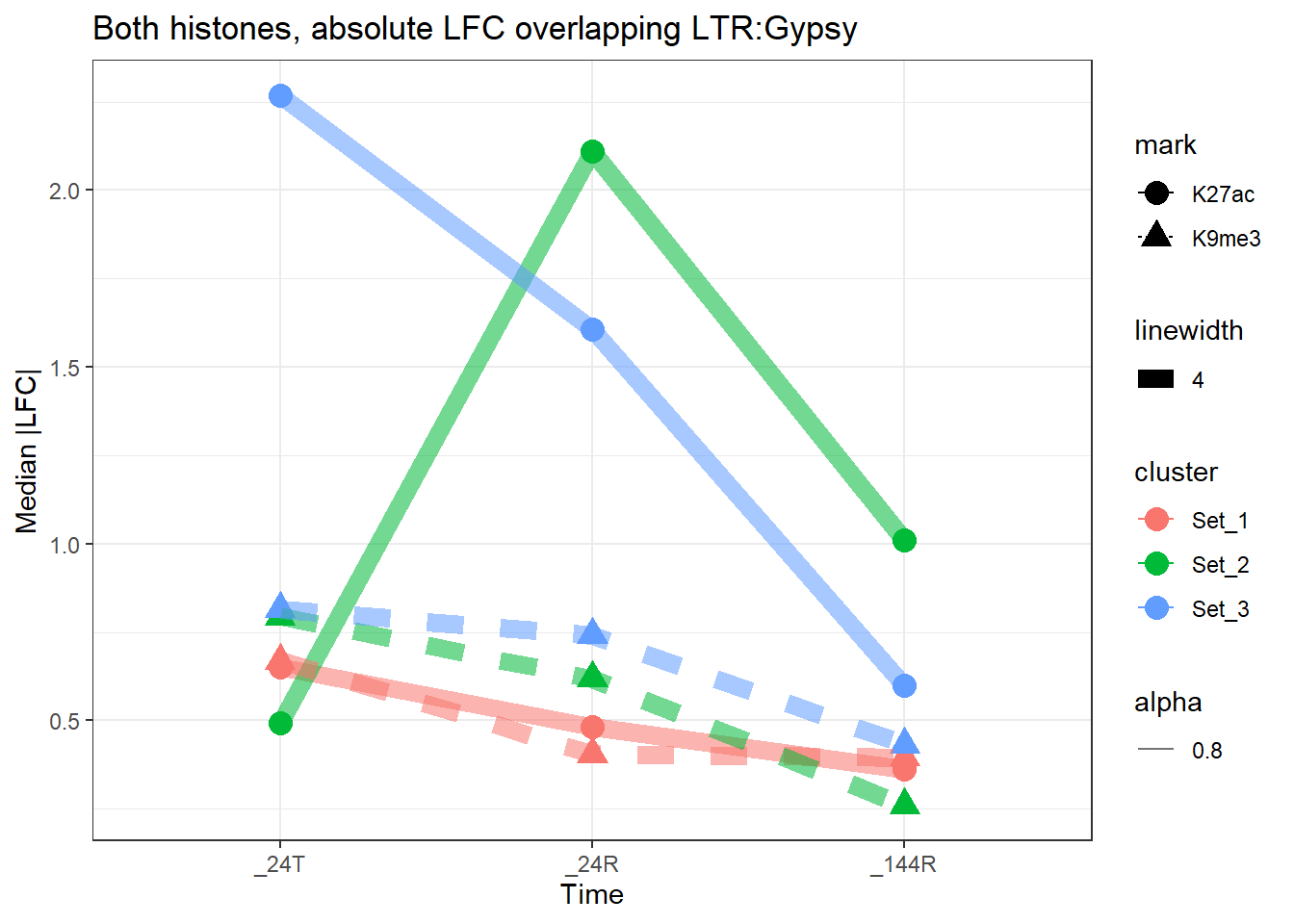
K27_K9_family_plot(LTR_RM_lfc_concordance, LTR_split_df,marks=c("K27ac","K9me3"), "LTR",repFam="LTR")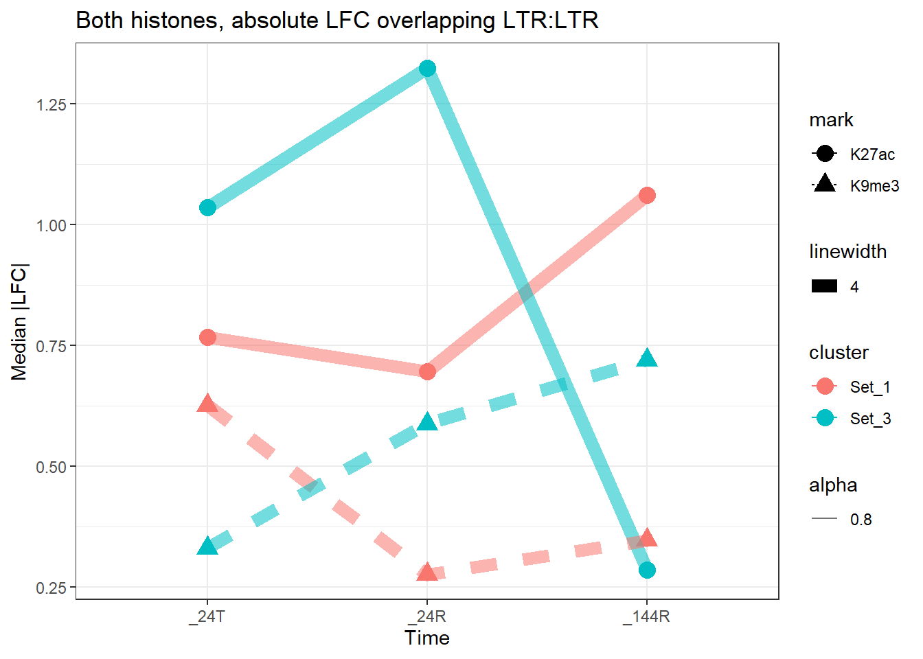
sessionInfo()R version 4.4.2 (2024-10-31 ucrt)
Platform: x86_64-w64-mingw32/x64
Running under: Windows 11 x64 (build 26200)
Matrix products: default
locale:
[1] LC_COLLATE=English_United States.utf8
[2] LC_CTYPE=English_United States.utf8
[3] LC_MONETARY=English_United States.utf8
[4] LC_NUMERIC=C
[5] LC_TIME=English_United States.utf8
time zone: America/Chicago
tzcode source: internal
attached base packages:
[1] grid stats4 stats graphics grDevices utils datasets
[8] methods base
other attached packages:
[1] smplot2_0.2.5 ggVennDiagram_1.5.4 ChIPseeker_1.42.1
[4] DT_0.33 ggrepel_0.9.6 rtracklayer_1.66.0
[7] genomation_1.38.0 plyranges_1.26.0 GenomicRanges_1.58.0
[10] GenomeInfoDb_1.42.3 IRanges_2.40.1 S4Vectors_0.44.0
[13] BiocGenerics_0.52.0 lubridate_1.9.4 forcats_1.0.0
[16] stringr_1.5.1 dplyr_1.1.4 purrr_1.1.0
[19] readr_2.1.5 tidyr_1.3.1 tibble_3.3.0
[22] ggplot2_3.5.2 tidyverse_2.0.0 workflowr_1.7.1
loaded via a namespace (and not attached):
[1] splines_4.4.2
[2] later_1.4.2
[3] BiocIO_1.16.0
[4] bitops_1.0-9
[5] ggplotify_0.1.2
[6] R.oo_1.27.1
[7] XML_3.99-0.18
[8] rpart_4.1.24
[9] lifecycle_1.0.4
[10] rstatix_0.7.2
[11] rprojroot_2.1.1
[12] MASS_7.3-65
[13] vroom_1.6.5
[14] processx_3.8.6
[15] lattice_0.22-7
[16] crosstalk_1.2.2
[17] backports_1.5.0
[18] magrittr_2.0.3
[19] Hmisc_5.2-3
[20] sass_0.4.10
[21] rmarkdown_2.29
[22] jquerylib_0.1.4
[23] yaml_2.3.10
[24] plotrix_3.8-4
[25] httpuv_1.6.16
[26] ggtangle_0.0.7
[27] cowplot_1.2.0
[28] DBI_1.2.3
[29] RColorBrewer_1.1-3
[30] abind_1.4-8
[31] zlibbioc_1.52.0
[32] R.utils_2.13.0
[33] RCurl_1.98-1.17
[34] yulab.utils_0.2.1
[35] nnet_7.3-20
[36] rappdirs_0.3.3
[37] git2r_0.36.2
[38] GenomeInfoDbData_1.2.13
[39] enrichplot_1.26.6
[40] tidytree_0.4.6
[41] codetools_0.2-20
[42] DelayedArray_0.32.0
[43] DOSE_4.0.1
[44] tidyselect_1.2.1
[45] aplot_0.2.8
[46] UCSC.utils_1.2.0
[47] farver_2.1.2
[48] matrixStats_1.5.0
[49] base64enc_0.1-3
[50] GenomicAlignments_1.42.0
[51] jsonlite_2.0.0
[52] Formula_1.2-5
[53] tools_4.4.2
[54] treeio_1.30.0
[55] TxDb.Hsapiens.UCSC.hg19.knownGene_3.2.2
[56] Rcpp_1.1.0
[57] glue_1.8.0
[58] gridExtra_2.3
[59] SparseArray_1.6.2
[60] mgcv_1.9-3
[61] xfun_0.52
[62] qvalue_2.38.0
[63] MatrixGenerics_1.18.1
[64] withr_3.0.2
[65] fastmap_1.2.0
[66] boot_1.3-32
[67] callr_3.7.6
[68] caTools_1.18.3
[69] digest_0.6.37
[70] timechange_0.3.0
[71] R6_2.6.1
[72] gridGraphics_0.5-1
[73] seqPattern_1.38.0
[74] colorspace_2.1-1
[75] GO.db_3.20.0
[76] gtools_3.9.5
[77] dichromat_2.0-0.1
[78] RSQLite_2.4.3
[79] R.methodsS3_1.8.2
[80] generics_0.1.4
[81] data.table_1.17.8
[82] httr_1.4.7
[83] htmlwidgets_1.6.4
[84] S4Arrays_1.6.0
[85] whisker_0.4.1
[86] pkgconfig_2.0.3
[87] gtable_0.3.6
[88] blob_1.2.4
[89] impute_1.80.0
[90] XVector_0.46.0
[91] htmltools_0.5.8.1
[92] carData_3.0-5
[93] pwr_1.3-0
[94] fgsea_1.32.4
[95] scales_1.4.0
[96] Biobase_2.66.0
[97] png_0.1-8
[98] ggfun_0.2.0
[99] knitr_1.50
[100] rstudioapi_0.17.1
[101] tzdb_0.5.0
[102] reshape2_1.4.4
[103] rjson_0.2.23
[104] checkmate_2.3.3
[105] nlme_3.1-168
[106] curl_7.0.0
[107] zoo_1.8-14
[108] cachem_1.1.0
[109] KernSmooth_2.23-26
[110] parallel_4.4.2
[111] foreign_0.8-90
[112] AnnotationDbi_1.68.0
[113] restfulr_0.0.16
[114] pillar_1.11.0
[115] vctrs_0.6.5
[116] gplots_3.2.0
[117] ggpubr_0.6.1
[118] promises_1.3.3
[119] car_3.1-3
[120] cluster_2.1.8.1
[121] htmlTable_2.4.3
[122] evaluate_1.0.5
[123] isoband_0.2.7
[124] GenomicFeatures_1.58.0
[125] cli_3.6.5
[126] compiler_4.4.2
[127] Rsamtools_2.22.0
[128] rlang_1.1.6
[129] crayon_1.5.3
[130] ggsignif_0.6.4
[131] labeling_0.4.3
[132] ps_1.9.1
[133] getPass_0.2-4
[134] plyr_1.8.9
[135] fs_1.6.6
[136] stringi_1.8.7
[137] gridBase_0.4-7
[138] BiocParallel_1.40.2
[139] Biostrings_2.74.1
[140] lazyeval_0.2.2
[141] GOSemSim_2.32.0
[142] Matrix_1.7-3
[143] BSgenome_1.74.0
[144] hms_1.1.3
[145] patchwork_1.3.2
[146] bit64_4.6.0-1
[147] KEGGREST_1.46.0
[148] SummarizedExperiment_1.36.0
[149] broom_1.0.9
[150] igraph_2.1.4
[151] memoise_2.0.1
[152] bslib_0.9.0
[153] ggtree_3.14.0
[154] fastmatch_1.1-6
[155] bit_4.6.0
[156] ape_5.8-1