Summit Files
Renee Matthews
2025-11-21
Last updated: 2025-11-21
Checks: 7 0
Knit directory: DXR_continue/
This reproducible R Markdown analysis was created with workflowr (version 1.7.1). The Checks tab describes the reproducibility checks that were applied when the results were created. The Past versions tab lists the development history.
Great! Since the R Markdown file has been committed to the Git repository, you know the exact version of the code that produced these results.
Great job! The global environment was empty. Objects defined in the global environment can affect the analysis in your R Markdown file in unknown ways. For reproduciblity it’s best to always run the code in an empty environment.
The command set.seed(20250701) was run prior to running
the code in the R Markdown file. Setting a seed ensures that any results
that rely on randomness, e.g. subsampling or permutations, are
reproducible.
Great job! Recording the operating system, R version, and package versions is critical for reproducibility.
Nice! There were no cached chunks for this analysis, so you can be confident that you successfully produced the results during this run.
Great job! Using relative paths to the files within your workflowr project makes it easier to run your code on other machines.
Great! You are using Git for version control. Tracking code development and connecting the code version to the results is critical for reproducibility.
The results in this page were generated with repository version 8a10509. See the Past versions tab to see a history of the changes made to the R Markdown and HTML files.
Note that you need to be careful to ensure that all relevant files for
the analysis have been committed to Git prior to generating the results
(you can use wflow_publish or
wflow_git_commit). workflowr only checks the R Markdown
file, but you know if there are other scripts or data files that it
depends on. Below is the status of the Git repository when the results
were generated:
Ignored files:
    Ignored:    .Rhistory
    Ignored:    .Rproj.user/
    Ignored:    data/Cormotif_data/
    Ignored:    data/DER_data/
    Ignored:    data/Other_paper_data/
    Ignored:    data/TE_annotation/
    Ignored:    data/alignment_summary.txt
    Ignored:    data/all_peak_final_dataframe.txt
    Ignored:    data/cell_line_info_.tsv
    Ignored:    data/full_summary_QC_metrics.txt
    Ignored:    data/motif_lists/
    Ignored:    data/number_frag_peaks_summary.txt

Untracked files:
    Untracked:  H3K27ac_all_regions_test.bed
    Untracked:  H3K27ac_consensus_clusters_test.bed
    Untracked:  analysis/Top2a_Top2b_expression.Rmd
    Untracked:  analysis/chromHMM.Rmd
    Untracked:  analysis/human_genome_composition.Rmd
    Untracked:  analysis/maps_and_plots.Rmd
    Untracked:  analysis/proteomics.Rmd
    Untracked:  code/making_analysis_file_summary.R
    Untracked:  other_analysis/

Unstaged changes:
    Modified:   analysis/Outlier_removal.Rmd
    Modified:   analysis/final_analysis.Rmd
    Modified:   analysis/multiQC_cut_tag.Rmd
Note that any generated files, e.g. HTML, png, CSS, etc., are not included in this status report because it is ok for generated content to have uncommitted changes.
These are the previous versions of the repository in which changes were
made to the R Markdown
(analysis/summit_files_processing.Rmd) and HTML
(docs/summit_files_processing.html) files. If you’ve
configured a remote Git repository (see ?wflow_git_remote),
click on the hyperlinks in the table below to view the files as they
were in that past version.
| File | Version | Author | Date | Message |
|---|---|---|---|---|
| Rmd | 8a10509 | reneeisnowhere | 2025-11-21 | wflow_publish("analysis/summit_files_processing.Rmd") |
| Rmd | f30fab7 | reneeisnowhere | 2025-11-19 | wflow_git_commit("analysis/summit_files_processing.Rmd") |
library(tidyverse)
library(GenomicRanges)
library(plyranges)
library(genomation)
library(readr)
library(rtracklayer)
library(stringr)
library(BiocParallel)
sampleinfo <- read_delim("data/sample_info.tsv", delim = "\t")
##Path to histone summit files
H3K27ac_dir <- "C:/Users/renee/Other_projects_data/DXR_data/final_data/summit_files/H3K27ac"
##pull all histone files together
H3K27ac_summit_files <- list.files(
path = H3K27ac_dir,
pattern = "\\.bed$",
recursive = TRUE,
full.names = TRUE
)
length(H3K27ac_summit_files)[1] 30# head(H3K27ac_summit_files)First steps: pulling in the information of Sets and locations Pulling in the summit files, concatenation of all summits into one large file
peakAnnoList_H3K27ac <- readRDS("data/motif_lists/H3K27ac_annotated_peaks.RDS")
H3K27ac_sets_gr <- lapply(peakAnnoList_H3K27ac, function(df) {
  as_granges(df)
})

read_summit <- function(file){
  peaks <- read.table(file,header = FALSE)
  colnames(peaks) <- c("chr","start","end","name","score")
  GRanges(
    seqnames = peaks$chr,
    ranges = IRanges(start=peaks$start, end = peaks$start),
    score=peaks$score,
    file=basename(file),
    Library_ID = stringr::str_remove(basename(file), "_FINAL_summits\\.bed$")
  )
}

all_H3K27ac_summits_list<- lapply(H3K27ac_summit_files, read_summit)
all_H3K27ac_summits_gr <- do.call(c, all_H3K27ac_summits_list)  # combine into one GRanges object
H3K27ac_lookup <- imap_dfr(peakAnnoList_H3K27ac[1:3], ~
  tibble(Peakid = .x@anno$Peakid, cluster = .y)
)
pick_best_summit_per_roi <- function(roi_gr, summit_gr, score_col = "signalValue") {
hits <- findOverlaps(roi_gr, summit_gr)
df <- data.frame(
roi_idx = queryHits(hits),
summit_idx = subjectHits(hits),
score = mcols(summit_gr)[[score_col]][subjectHits(hits)]
)
# Pick summit with highest score for each ROI
best <- df %>%
group_by(roi_idx) %>%
slice_max(order_by = score, n = 1) %>%
ungroup()
# Build the final GRanges object
best_summits <- summit_gr[best$summit_idx]
best_summits$ROI_name <- roi_gr$Peakid[best$roi_idx]
best_summits
}
#
# best_summits <- pick_best_summit_per_roi(
# ROIs, highest_summits_long_gr, score_col = "peakHeight"
# )pick_center_summit <- function(roi_gr, summit_gr) {
hits <- findOverlaps(roi_gr, summit_gr)
df <- data.frame(
roi_idx = queryHits(hits),
summit_idx = subjectHits(hits),
dist_to_center = abs(
start(summit_gr)[subjectHits(hits)] -
round((start(roi_gr)[queryHits(hits)] + end(roi_gr)[queryHits(hits)]) / 2)
)
)
best <- df %>%
group_by(roi_idx) %>%
slice_min(order_by = dist_to_center, n = 1) %>%
ungroup()
best_summits <- summit_gr[best$summit_idx]
best_summits$ROI_name <- roi_gr$Peakid[best$roi_idx]
best_summits
}pick_consensus_summit <- function(roi_gr, summit_gr, score_col = "score") {
# Find which summits overlap each ROI
hits <- findOverlaps(roi_gr, summit_gr)
df <- data.frame(
roi_idx = queryHits(hits),
summit_idx = subjectHits(hits),
summit_pos = start(summit_gr)[subjectHits(hits)],
score = mcols(summit_gr)[[score_col]]
)
# Count frequency per summit position within each ROI
freq_df <- df %>%
group_by(roi_idx, summit_pos) %>%
summarise(
freq = n(),
max_score = max(score),
.groups = "drop"
)
# Pick the summit with highest frequency; break ties with max score
best <- freq_df %>%
group_by(roi_idx) %>%
slice_max(order_by = freq, n = 1, with_ties = TRUE) %>%
slice_max(order_by = max_score, n = 1) %>%
ungroup()
# Map back to original GRanges
best_idx <- df$summit_idx[match(
paste0(best$roi_idx, "_", best$summit_pos),
paste0(df$roi_idx, "_", df$summit_pos)
)]
final_summits <- summit_gr[best_idx]
final_summits$ROI_name <- roi_gr$Peakid[best$roi_idx]
final_summits
}Analysis of all summit files, no grouping
first creating summit clusters that are around 100bps across all summit files
#  Merge summits within 100 bp clusters but keep metadata
# ------------------------
# 1 Reduce with revmap to keep track of original indices

clusters <- GenomicRanges::reduce(all_H3K27ac_summits_gr, min.gapwidth = 100,
                   ignore.strand = TRUE, with.revmap = TRUE)

# 2 For each cluster, pick the highest-score summit
scores <- mcols(all_H3K27ac_summits_gr)$score

revmap <- clusters$revmap

# Compute the highest-score index per cluster
highest_idx <- sapply(revmap, function(idx) idx[which.max(scores[idx])])

# Subset GRanges once
highest_per_cluster_gr <- all_H3K27ac_summits_gr[highest_idx]


# ------------------------
# 3 Count merged summits per ROI
# ------------------------
ROIs <- H3K27ac_sets_gr$all_H3K27ac  # your ROI GRanges

# Optimized counting
roi_counts <- countOverlaps(ROIs, highest_per_cluster_gr)
mcols(ROIs)$merged_summit_count <- roi_counts

# ------------------------
# 5 Map ROIs to clusters with sample info
# ------------------------
overlaps <- findOverlaps(ROIs, highest_per_cluster_gr)

roi_hits_df <- as.data.frame(overlaps) %>%
  mutate(
    Peakid = ROIs$Peakid[queryHits],
    Library_ID = mcols(highest_per_cluster_gr)$Library_ID[subjectHits],
    score = mcols(highest_per_cluster_gr)$score[subjectHits],
    file = mcols(highest_per_cluster_gr)$file[subjectHits]
  ) %>%
  left_join(sampleinfo, by = c("Library_ID" = "Library ID"))

## initualize count column on ROI df
mcols(ROIs)$summit_count <- 0

# Tabulate counts
counts <- table(queryHits(overlaps))
mcols(ROIs)$summit_count[as.numeric(names(counts))] <- as.numeric(counts)

# Convert to dataframe for plotting
roi_counts_df <- as.data.frame(ROIs) %>%
  select(Peakid, seqnames, start, end, summit_count) %>%
  mutate(roi_size=end-start)

# Optional: add Set / cluster info
roi_counts_df <- roi_counts_df %>%
  left_join(H3K27ac_lookup, by = "Peakid")
# ------------------------
# 6 Optional: add Set/cluster info per ROI
# ------------------------
roi_hits_df <- roi_hits_df %>%
  left_join(H3K27ac_lookup, by = "Peakid")

# Now roi_hits_df is ready for plotting or analysis:
# Columns include Peakid, ROI coordinates, Library_ID, score, file, Individual, Treatment, Timepoint, cluster


# Optional: add sample info
roi_hits_df <- as.data.frame(overlaps) %>%
  mutate(
    Peakid = ROIs$Peakid[queryHits],
    Library_ID = mcols(all_H3K27ac_summits_gr)$Library_ID[subjectHits],
    score = mcols(all_H3K27ac_summits_gr)$score[subjectHits],
    file = mcols(all_H3K27ac_summits_gr)$file[subjectHits]
  ) %>%
  left_join(sampleinfo, by = c("Library_ID" = "Library ID"))
Plotting some summits from the first process
ROIs %>%
  as.data.frame() %>%
  # dplyr::filter(merged_summit_count==1) %>%
  left_join(H3K27ac_lookup, by = "Peakid") %>%  # make sure join key matches
  filter(!is.na(cluster)) %>%
  ggplot(aes(x = cluster, y = merged_summit_count)) +
  geom_jitter(width = 0.2, height = 0, alpha = 0.6, size = 2, color = "steelblue") +
  theme_bw() +
  xlab("Set") +
  ylab("Number of merged summits per ROI") +
  ggtitle("Distribution of merged summit counts by Set")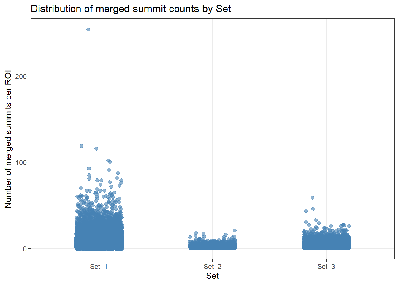
roi_counts_df %>%
  ggplot(aes(x = summit_count)) +
  geom_histogram(binwidth = 1, fill="steelblue", color="black") +
  theme_bw() +
  xlab("Number of summits per ROI") +
  ylab("Number of ROIs")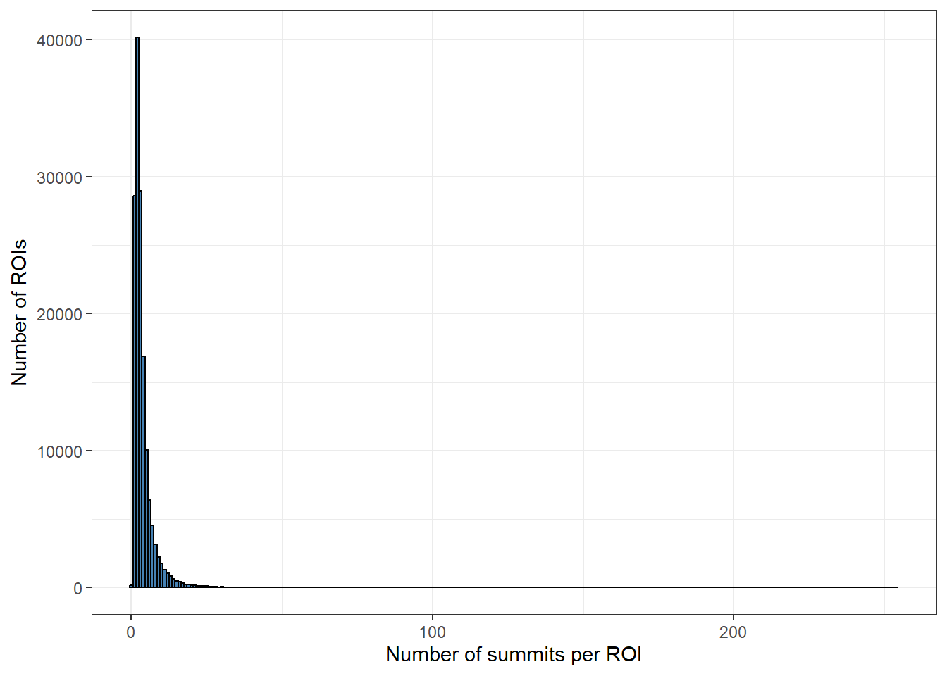
roi_counts_df %>%
  ggplot(aes(x = summit_count)) +
  geom_histogram(binwidth = 1, fill="steelblue", color="black") +
  theme_bw() +
  xlab("Number of summits per ROI") +
  ylab("Number of ROIs")+
  ggtitle("Zoomed in summit per ROI")+
  coord_cartesian(xlim=c(0,50))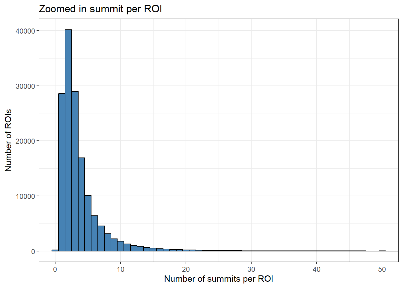
roi_counts_df %>%
  # group_by(Peakid) %>% tally #%>%
  # left_join(H3K27ac_lookup) %>%
  ggplot(aes(x = roi_size, y = summit_count)) +
  geom_point(alpha = 0.5) +
  geom_smooth(method = "lm", se = FALSE) +
  labs(
    x = "ROI size (bp)",
    y = "# of summits",
    title = "Relationship between ROI size and # of Summit clusters"
  ) +
  theme_classic()#+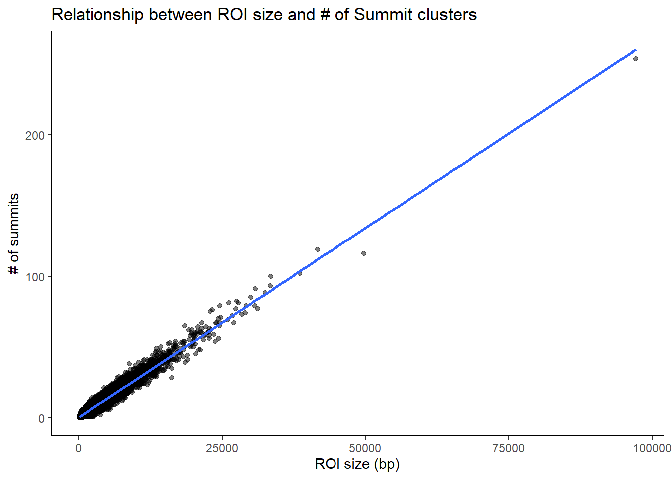
  # coord_cartesian(xlim=c(-1,400), ylim=c(0,10))

roi_counts_df %>%
  # group_by(Peakid) %>% tally #%>%
  # left_join(H3K27ac_lookup) %>%
  ggplot(aes(x = roi_size, y = summit_count)) +
  geom_point(alpha = 0.5) +
  geom_smooth(method = "lm", se = FALSE) +
  labs(
    x = "ROI size (bp)",
    y = "# of summits",
    title = "Zoomed in Relationship between ROI size and # of Summit clusters"
  ) +
  theme_classic()+
  coord_cartesian(xlim=c(-1,800), ylim=c(0,10))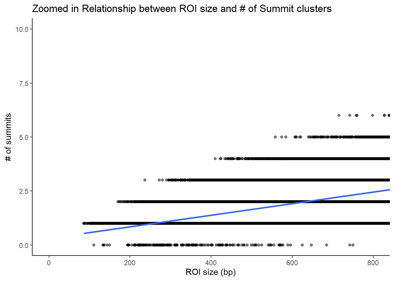
Merging strategies!
This is now the place I will take my files and now try to apply the same merging strategy as I did the peaks merging strategy. Step 1: reduce all trt-time summits within 100 bp
###Adding in sampleinfo dataframe
meta <- as.data.frame(mcols(all_H3K27ac_summits_gr))
meta2 <- meta %>%
  left_join(., sampleinfo, by=c("Library_ID"="Library ID"))

mcols(all_H3K27ac_summits_gr) <- meta2

mcols(all_H3K27ac_summits_gr)$group <-
  paste(all_H3K27ac_summits_gr$Treatment,
        all_H3K27ac_summits_gr$Timepoint,
        sep = "_")

###now splitting into grouped granges

gr_by_group <- split(all_H3K27ac_summits_gr,
                                    all_H3K27ac_summits_gr$group)
# gr_by_group <- as(gr_by_group, "CompressedGRangesList")
### now reducing within some width by 100 bp with revmap
groups <- unique(all_H3K27ac_summits_gr$group)

reduced_groups <- lapply(groups, function(g) {
  gr_sub <- all_H3K27ac_summits_gr[all_H3K27ac_summits_gr$group == g]
  GenomicRanges::reduce(gr_sub, min.gapwidth = 100, ignore.strand = TRUE, with.revmap = TRUE)
})

reduced_groups_200 <- lapply(groups, function(g) {
  gr_sub <- all_H3K27ac_summits_gr[all_H3K27ac_summits_gr$group == g]
  GenomicRanges::reduce(gr_sub, min.gapwidth = 200, ignore.strand = TRUE, with.revmap = TRUE)
})

reduced_groups_300 <- lapply(groups, function(g) {
  gr_sub <- all_H3K27ac_summits_gr[all_H3K27ac_summits_gr$group == g]
  GenomicRanges::reduce(gr_sub, min.gapwidth = 300, ignore.strand = TRUE, with.revmap = TRUE)
})

reduced_groups_400 <- lapply(groups, function(g) {
  gr_sub <- all_H3K27ac_summits_gr[all_H3K27ac_summits_gr$group == g]
  GenomicRanges::reduce(gr_sub, min.gapwidth = 400, ignore.strand = TRUE, with.revmap = TRUE)
})

names(reduced_groups) <- groups
names(reduced_groups_200) <- groups
names(reduced_groups_300) <- groups
names(reduced_groups_400) <- groups

# redux_main_100 <- sum(sapply(reduced_groups, length))
# redux_main_200 <- sum(sapply(reduced_groups_200, length))
# redux_main_300 <- sum(sapply(reduced_groups_300, length))
# redux_main_400 <- sum(sapply(reduced_groups_400, length))
Plotting effect of reduction bp number on total number of clusters
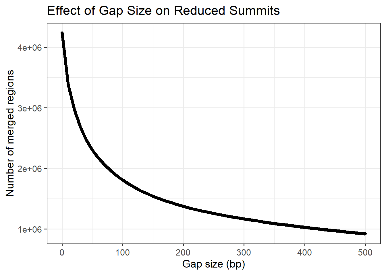
gap_sizes <- seq(0, 500, by = 10)


# Function to apply reduce for each gap and return counts
results <- lapply(gap_sizes, function(g) {
  reduced <- GenomicRanges::reduce(all_H3K27ac_summits_gr, min.gapwidth = g)
  data.frame(gap = g, n_regions = length(reduced))
})

# Combine results
min_gap_summary <- bind_rows(results)

ggplot(min_gap_summary, aes(x = gap, y= n_regions))+
  geom_line(linewidth=2)+
  geom_point()+
  theme_bw(base_size=14)+
  labs(
    title = "Effect of Gap Size on Reduced Summits",
    x = "Gap size (bp)",
    y = "Number of merged regions"
  )
# Function to pick highest summit per cluster from a reduced GRanges list
get_highest_per_group <- function(reduced_groups, orig_summits_gr, group_col = "group") {

  groups <- names(reduced_groups)
  highest_per_group <- vector("list", length(reduced_groups))
  names(highest_per_group) <- groups

  for(i in seq_along(reduced_groups)) {
    gr <- reduced_groups[[i]]

    # original summits for this group
    orig <- orig_summits_gr[mcols(orig_summits_gr)[[group_col]] == groups[i]]
    scores <- orig$score

    # revmap is a CompressedIntegerList
    revmap <- mcols(gr)$revmap

    # skip if revmap is NULL
    if(is.null(revmap)) next

    # unlist all indices once
    all_idx <- unlist(revmap, use.names = FALSE)

    # repeat cluster index for each element in revmap
    cluster_idx <- rep(seq_along(revmap), times = elementNROWS(revmap))

    # scores for all indices
    all_scores <- scores[all_idx]

    # For each cluster, pick the index of the max score
    max_idx_per_cluster <- tapply(seq_along(all_scores), cluster_idx, function(ii) {
      ii[which.max(all_scores[ii])]
    })

    # Convert back to original indices
    orig_idx <- all_idx[unlist(max_idx_per_cluster)]

    # subset original GRanges
    highest_per_group[[i]] <- orig[orig_idx]
  }

  # Flatten any nested GRangesList
  flatten_gr <- function(x) {
    if (inherits(x, "GRanges")) return(x)
    if (inherits(x, "GRangesList")) return(unlist(x, use.names = FALSE))
    if (is.list(x)) return(do.call(c, lapply(x, flatten_gr)))
    stop("Unexpected object type")
  }

  highest_summits_gr <- flatten_gr(highest_per_group)

  # Return as long GRanges with group column
  highest_summits_df <- bind_rows(
    lapply(names(highest_per_group), function(gr_name) {
      as.data.frame(highest_per_group[[gr_name]]) %>%
        mutate(group = gr_name)
    })
  )

  highest_summits_long_gr <- highest_summits_df %>% GRanges()

  return(highest_summits_long_gr)
}
reduced_sets <- list(
"100bp" = reduced_groups,
"200bp" = reduced_groups_200,
"300bp" = reduced_groups_300,
"400bp" = reduced_groups_400
)
highest_summits_all <- lapply(reduced_sets, get_highest_per_group, orig_summits_gr = all_H3K27ac_summits_gr)Looking at number of summits across groups as a function of min.gap number
##Compute counts per group for each reduced set
summit_counts_group <- lapply(names(highest_summits_all), function(gap_name) {
gr <- highest_summits_all[[gap_name]]
# make sure group column exists
if(!"group" %in% colnames(mcols(gr))) stop("GRanges must have 'group' column")
df <- as.data.frame(gr) %>%
count(group, name = "n_summits") %>%
mutate(gap = gap_name)
return(df)
}) %>% bind_rows()
ggplot(summit_counts_group, aes(x = gap, y = n_summits, group = group, color = group)) +
geom_line(size = 1.2) +
geom_point(size = 3) +
theme_classic(base_size = 14) +
labs(
title = "Effect of min-gap width on number of highest summits per group",
x = "Min-gap width (bp)",
y = "Number of highest summits",
color = "Group"
) +
theme(axis.text.x = element_text(angle = 45, hjust = 1))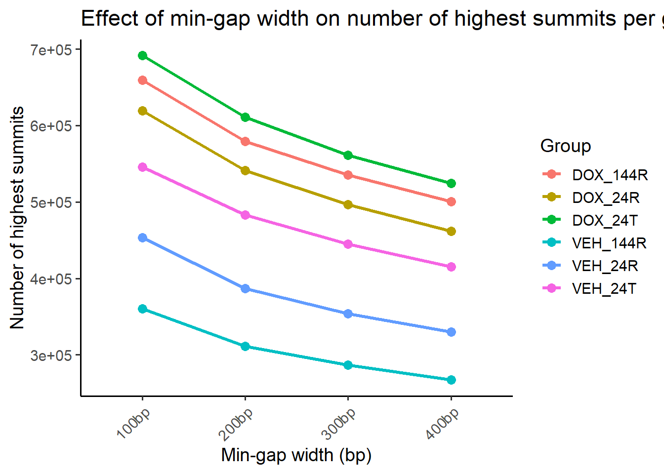 ### Summit average per ROI What is the average number of summits per ROI
as a function of min.gapwidth
### Summit average per ROI What is the average number of summits per ROI
as a function of min.gapwidth
double_reduce_summits <- function(summits_gr, ROIs, groups,
                                  min_gap_within_seq = c(100,200,300),
                                  min_gap_across_seq = c(100,200,300),
                                  BPPARAM = MulticoreParam(4)) {

  # Pre-split summits by group to avoid repeated subsetting
  summits_by_group <- split(summits_gr, summits_gr$group)

  # Create all gap combinations
  gap_combos <- expand.grid(min_gap_within = min_gap_within_seq,
                            min_gap_across = min_gap_across_seq,
                            stringsAsFactors = FALSE)

  # Apply in parallel for each combination
  results <- bplapply(seq_len(nrow(gap_combos)), function(i) {
    g1 <- gap_combos$min_gap_within[i]
    g2 <- gap_combos$min_gap_across[i]

    # -----------------
    # Step 1: Reduce within group
    # -----------------
    highest_per_group <- lapply(groups, function(grp) {
      gr_sub <- summits_by_group[[grp]]
      if(length(gr_sub) == 0) return(NULL)

      # reduce within group with revmap
      red <- GenomicRanges::reduce(gr_sub, min.gapwidth = g1, ignore.strand = TRUE, with.revmap = TRUE)
      revmap <- mcols(red)$revmap
      if(length(revmap) == 0) return(NULL)

      # pick highest score per cluster
      cluster_idx <- rep(seq_along(revmap), times = elementNROWS(revmap))
      all_idx <- unlist(revmap, use.names = FALSE)
      all_scores <- gr_sub$score[all_idx]
      max_idx_per_cluster <- tapply(seq_along(all_scores), cluster_idx, function(ii) {
        ii[which.max(all_scores[ii])]
      })
      gr_sub[all_idx[unlist(max_idx_per_cluster)]]
    })

    highest_per_group <- highest_per_group[!sapply(highest_per_group, is.null)]

    # -----------------
    # Step 2: Merge across groups
    # -----------------
    if(length(highest_per_group) == 0) return(NULL)
    all_highest <- do.call(c, highest_per_group)
    consensus <- GenomicRanges::reduce(all_highest, min.gapwidth = g2, ignore.strand = TRUE)

    # -----------------
    # Step 3: Count summits per ROI (vectorized)
    # -----------------
    hits <- findOverlaps(ROIs, consensus)
    counts <- as.data.frame(table(queryHits(hits)))
    colnames(counts) <- c("ROI_idx", "n_summits")
    counts$ROI_idx <- as.integer(as.character(counts$ROI_idx))
    counts$min_gap_within <- g1
    counts$min_gap_across <- g2
    counts
  }, BPPARAM = BPPARAM)

  # Combine results
  results_df <- bind_rows(results)

  return(results_df)
}
BPPARAM <- SnowParam(workers = 4, type = "SOCK")
register(BPPARAM)
heatmap_data <- double_reduce_summits(
summits_gr = all_H3K27ac_summits_gr,
ROIs = H3K27ac_sets_gr$all_H3K27ac,
groups = unique(all_H3K27ac_summits_gr$group),
min_gap_within_seq = c(100,200,300,400),
min_gap_across_seq = c(100,200,300,400),
BPPARAM = BPPARAM
)
heatmap_avg <- heatmap_data %>%
group_by(min_gap_within, min_gap_across) %>%
summarise(mean_summits = mean(n_summits, na.rm = TRUE), .groups = "drop")ggplot(heatmap_avg, aes(x = factor(min_gap_within),
y = factor(min_gap_across),
fill = mean_summits)) +
geom_tile(color = "white") +
geom_text(aes(label = round(mean_summits, 1)), color = "black", size = 4) +
scale_fill_viridis_c(option = "plasma") +
labs(
x = "Within-group min-gap (bp)",
y = "Across-group min-gap (bp)",
fill = "Mean # summits per ROI",
title = "Effect of min-gap width on summits per ROI"
) +
theme_minimal(base_size = 14) +
theme(axis.text.x = element_text(angle = 45, hjust = 1))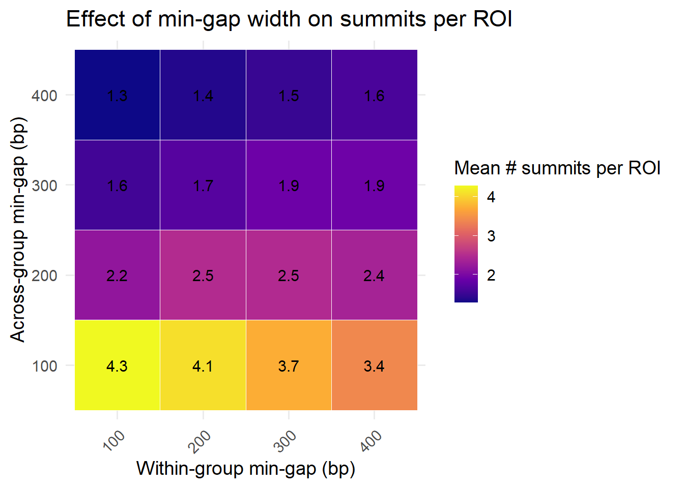
after i figure my final min.gaps, here is where the places are
# --- Step 1: Reduce within groups and pick highest summit per cluster ---
get_highest_per_group <- function(summits_gr, groups = NULL, min_gap_within = 100) {

  if(is.null(groups)) {
    groups <- unique(summits_gr$group)
  }

  highest_per_group <- lapply(groups, function(grp) {
    gr_sub <- summits_gr[summits_gr$group == grp]
    if(length(gr_sub) == 0) return(NULL)

    # Reduce within group
    reduced <- GenomicRanges::reduce(gr_sub, min.gapwidth = min_gap_within, ignore.strand = TRUE, with.revmap = TRUE)

    # Pick highest scoring summit per cluster
    revmap <- reduced$revmap
    scores <- gr_sub$score

    all_idx <- unlist(revmap, use.names = FALSE)
    cluster_idx <- rep(seq_along(revmap), times = elementNROWS(revmap))
    all_scores <- scores[all_idx]

    max_idx_per_cluster <- tapply(seq_along(all_scores), cluster_idx, function(ii) {
      ii[which.max(all_scores[ii])]
    })

    orig_idx <- all_idx[unlist(max_idx_per_cluster)]

    gr_sub[orig_idx]
  })

  # Flatten list of GRanges
  highest_per_group <- do.call(c, highest_per_group)
  return(highest_per_group)
}

# --- Step 2: Reduce across groups to get final consensus ---
get_consensus_summits <- function(highest_per_group_gr, min_gap_across = 400) {

  # Reduce across groups
  reduced <- GenomicRanges::reduce(highest_per_group_gr, min.gapwidth = min_gap_across, ignore.strand = TRUE, with.revmap = TRUE)

  # Pick highest scoring summit per cluster across all groups
  revmap <- reduced$revmap
  scores <- highest_per_group_gr$score

  all_idx <- unlist(revmap, use.names = FALSE)
  cluster_idx <- rep(seq_along(revmap), times = elementNROWS(revmap))
  all_scores <- scores[all_idx]

  max_idx_per_cluster <- tapply(seq_along(all_scores), cluster_idx, function(ii) {
    ii[which.max(all_scores[ii])]
  })

  orig_idx <- all_idx[unlist(max_idx_per_cluster)]

  highest_per_group_gr[orig_idx]
}

add_ROI_to_consensus <- function(consensus_gr, ROIs_gr) {

  hits <- findOverlaps(consensus_gr, ROIs_gr)

  df <- data.frame(
    summit_chr  = seqnames(consensus_gr)[queryHits(hits)],
    summit_pos  = start(consensus_gr)[queryHits(hits)],
    summit_score = consensus_gr$score[queryHits(hits)],
    Peakid      = ROIs_gr$Peakid[subjectHits(hits)],
    roi_start   = start(ROIs_gr)[subjectHits(hits)],
    roi_end     = end(ROIs_gr)[subjectHits(hits)]
  )

  df %>%
    mutate(rel_pos = (summit_pos - roi_start)/(roi_end - roi_start),
           roi_center = roi_start + (roi_end - roi_start)/2,
           dist_center = summit_pos - roi_center)
}
highest_100 <- get_highest_per_group(all_H3K27ac_summits_gr, min_gap_within = 100)
final_consensus <- get_consensus_summits(highest_100, min_gap_across = 400)
final_df_100_400 <- add_ROI_to_consensus(final_consensus, H3K27ac_sets_gr$all_H3K27ac)
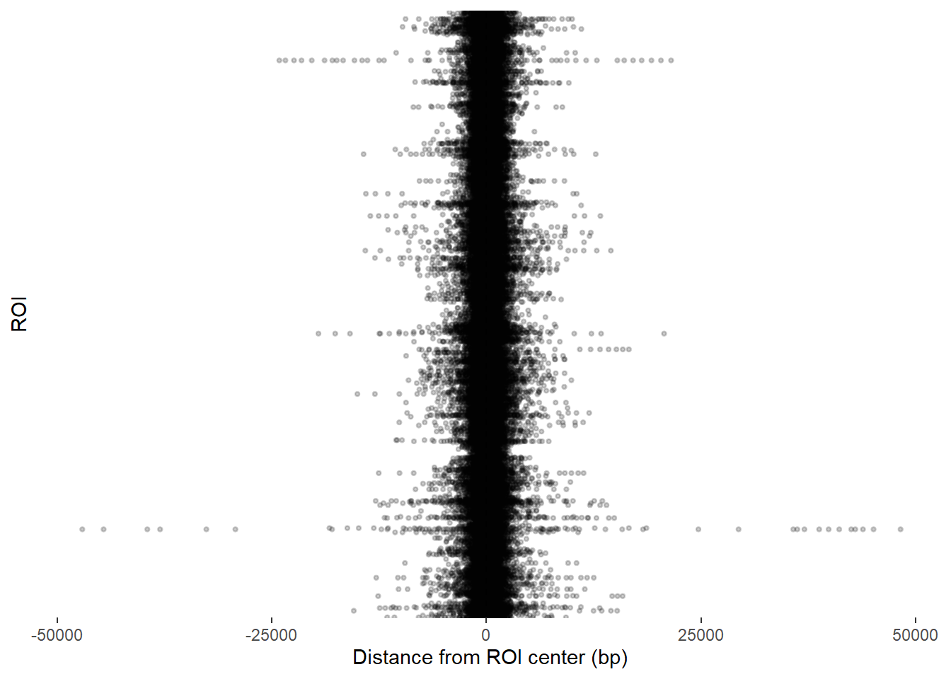
ggplot(final_df_100_400, aes(x = dist_center, y = Peakid)) +
ggrastr::geom_point_rast(size = 0.6, alpha = 0.2) +
geom_vline(xintercept = 0, linetype = "dashed") + # ROI center
labs(
x = "Distance from ROI center (bp)",
y = "ROI",
color = "Group"
) +
# theme_minimal() +
theme(
axis.text.y = element_blank(),
axis.ticks.y = element_blank()
)
final_df_100_400 %>%
  group_by(Peakid) %>%
  slice_max(summit_score) %>%
ggplot(., aes(x = dist_center, y = Peakid)) +
  ggrastr::geom_point_rast(size = 0.6, alpha = 0.2) +
  geom_vline(xintercept = 0, linetype = "dashed") +  # ROI center
  geom_vline(xintercept = 500, linetype = "dashed",color="red") +  # left 500
  geom_vline(xintercept = -500, linetype = "dashed",color="red") +  # right 500
  geom_vline(xintercept = 250, linetype = "dashed",color="yellow") +  # left 500
  geom_vline(xintercept = -250, linetype = "dashed",color="yellow") +  # right 500

  labs(
    x = "Distance from ROI center (bp)",
    y = "ROI",
    color = "Group"
  ) +
  # theme_minimal() +
  theme(
    axis.text.y = element_blank(),
    axis.ticks.y = element_blank()
  )+
 coord_cartesian(xlim=c(-2000,2000))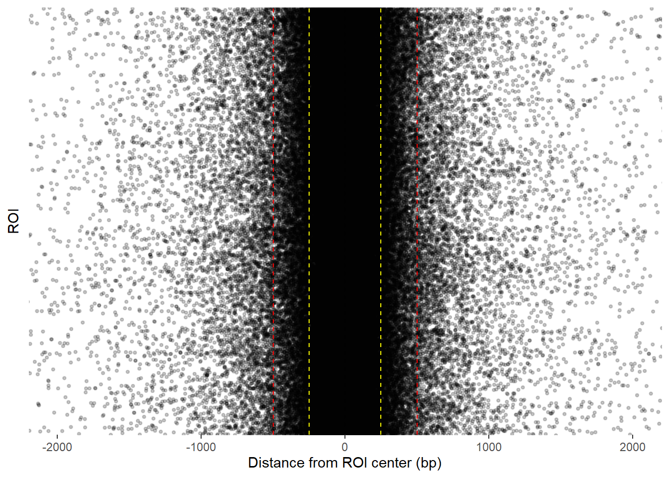
final_df_100_400 %>%
  group_by(Peakid) %>%
  slice_max(summit_score) %>%
ggplot(., aes(x = dist_center)) +
  geom_density()+
  geom_vline(xintercept = 0, linetype = "dashed") +  # ROI center
  geom_vline(xintercept = 500, linetype = "dashed",color="red") +  # left 500
  geom_vline(xintercept = -500, linetype = "dashed",color="red") +  # right 500
  geom_vline(xintercept = 250, linetype = "dashed",color="blue") +  # left 500
  geom_vline(xintercept = -250, linetype = "dashed",color="blue") +  # right 500
 coord_cartesian(xlim=c(-2000,2000))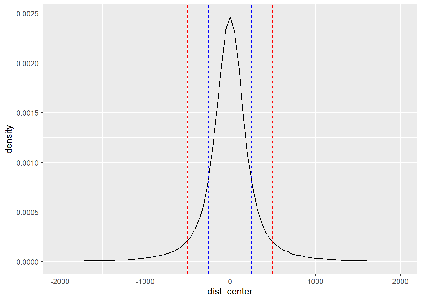
highest_200 <- get_highest_per_group(all_H3K27ac_summits_gr, min_gap_within = 200)

final_consensus2 <- get_consensus_summits(highest_200, min_gap_across = 400)

final_df_200_400 <- add_ROI_to_consensus(final_consensus2, H3K27ac_sets_gr$all_H3K27ac)


ggplot(final_df_100_400, aes(x = dist_center, y = Peakid)) +
  ggrastr::geom_point_rast(size = 0.6, alpha = 0.2) +
  geom_vline(xintercept = 0, linetype = "dashed", color="green") +  # ROI center
  geom_vline(xintercept = 500, linetype = "dashed",color="red") +  # left 500
  geom_vline(xintercept = -500, linetype = "dashed",color="red") +  # right 500
  labs(
    x = "Distance from ROI center (bp)",
    y = "ROI",
    color = "Group"
  ) +
  # theme_minimal() +
  theme(
    axis.text.y = element_blank(),
    axis.ticks.y = element_blank()
  )+coord_cartesian(xlim=c(-2000,2000))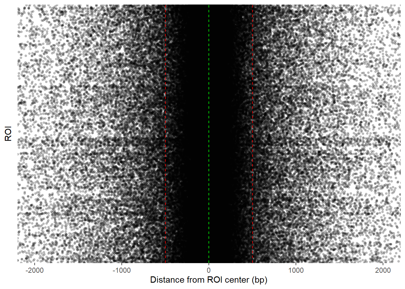
function get highest scoring summit clustered by group:
#' Get highest summit per reduced cluster per group using plyranges
#'
#' @param gr GRanges with metadata columns: group, score
#' @param min_gap numeric, minimum gap width to merge summits
#' @param ignore.strand logical, whether to ignore strand when reducing
#'
#' @return GRanges of highest scoring summit per reduced cluster per group
get_highest_summits_with_cluster_id <- function(gr, min_gap = 100, ignore.strand = TRUE) {

  gr %>%
    # Reduce summits per group
    group_by(group) %>%
    reduce_ranges(min_gap = min_gap, ignore.strand = ignore.strand, with_revmap = TRUE) %>%
    # Add a cluster_id based on row_number()
    mutate(cluster_id = paste0(group, "_cluster_", row_number())) %>%
    # join back original summits
    join_overlap_inner(gr, suffix = c(".cluster", ".orig")) %>%
    # slice max per cluster_id
    group_by(cluster_id) %>%
    slice_max(score.orig, with_ties = FALSE) %>%
    ungroup() %>%
    # select only the original summit coordinates
    select(seqnames, start = start.orig, end = end.orig, score = score.orig,
           group, cluster_id)
}
function reduce_and_pick_highest
#### this quickly reduces any granges summit  collection by the gap that is passed in the function. It returns the highest scoring summit from the cluster of summits.
reduce_and_pick_highest <- function(gr, gap = 100) {

  # Preextract score once
  sc <- gr$score

  # Fast reduce with revmap
  red <- GenomicRanges::reduce(
    gr,
    min.gapwidth = gap,
    ignore.strand = TRUE,
    with.revmap = TRUE
  )

  # This is vectorized and very fast
  idx_list <- red$revmap

  # Pick highest-scoring summit within each cluster
  sel <- IntegerList(
    lapply(idx_list, function(idx) idx[which.max(sc[idx])])
  )

  # Convert IntegerList → integer vector
  best_idx <- unlist(sel, use.names = FALSE)

  # Subset original GRanges
  gr[best_idx]
}
redux_100 <- reduce_and_pick_highest(all_H3K27ac_summits_gr, gap = 100)
redux_200 <- reduce_and_pick_highest(all_H3K27ac_summits_gr, gap = 200)
redux_300 <- reduce_and_pick_highest(all_H3K27ac_summits_gr, gap = 300)
redux_Peak_100 <- add_ROI_to_consensus(redux_100, H3K27ac_sets_gr$all_H3K27ac)
redux_Peak_200 <- add_ROI_to_consensus(redux_200, H3K27ac_sets_gr$all_H3K27ac)
redux_Peak_300 <- add_ROI_to_consensus(redux_300, H3K27ac_sets_gr$all_H3K27ac)ggplot(redux_Peak_100, aes(x = dist_center, y = Peakid)) +
ggrastr::geom_point_rast(size = 0.6, alpha = 0.2) +
geom_vline(xintercept = 0, linetype = "dashed") + # ROI center
geom_vline(xintercept = 500, linetype = "dashed",color="red") + # left 500
geom_vline(xintercept = -500, linetype = "dashed",color="red") + # right 500
labs(
x = "Distance from ROI center (bp)",
y = "ROI",
color = "Group"
) +
# theme_minimal() +
theme(
axis.text.y = element_blank(),
axis.ticks.y = element_blank()
)+
ggtitle("Only single reduction 100bp")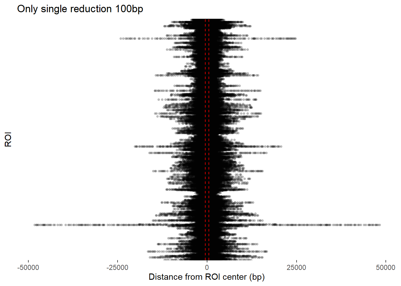
ggplot(redux_Peak_200, aes(x = dist_center, y = Peakid)) +
  ggrastr::geom_point_rast(size = 0.6, alpha = 0.2) +
  geom_vline(xintercept = 0, linetype = "dashed") +  # ROI center
  geom_vline(xintercept = 500, linetype = "dashed",color="red") +  # left 500
  geom_vline(xintercept = -500, linetype = "dashed",color="red") +  # right 500
  labs(
    x = "Distance from ROI center (bp)",
    y = "ROI",
    color = "Group"
  ) +
  # theme_minimal() +
  theme(
    axis.text.y = element_blank(),
    axis.ticks.y = element_blank()
  )+
  ggtitle("Only single reduction 200bp")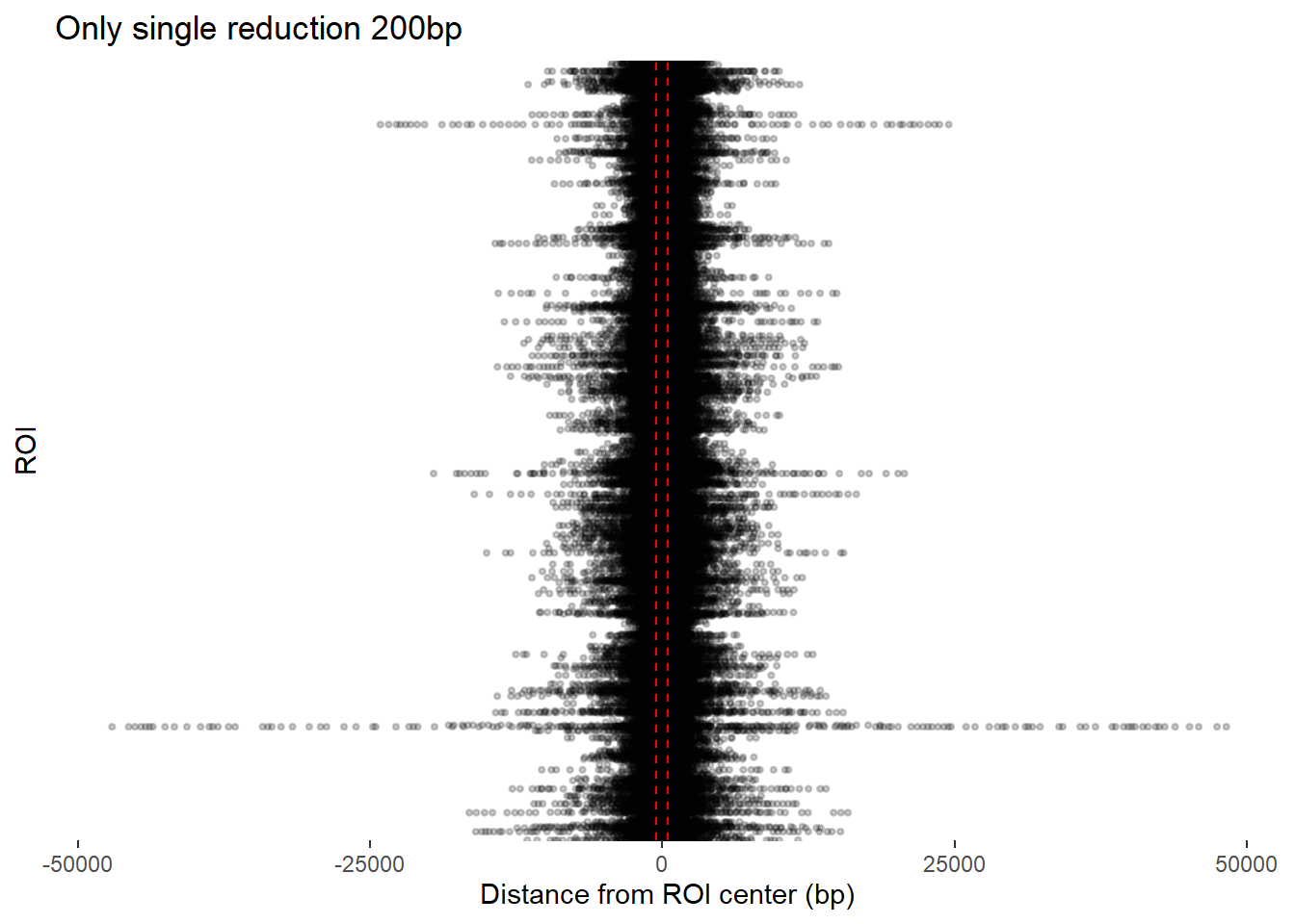
ggplot(redux_Peak_300, aes(x = dist_center, y = Peakid)) +
  ggrastr::geom_point_rast(size = 0.6, alpha = 0.2) +
  geom_vline(xintercept = 0, linetype = "dashed") +  # ROI center
  geom_vline(xintercept = 500, linetype = "dashed",color="red") +  # left 500
  geom_vline(xintercept = -500, linetype = "dashed",color="red") +  # right 500
  labs(
    x = "Distance from ROI center (bp)",
    y = "ROI",
    color = "Group"
  ) +
  # theme_minimal() +
  theme(
    axis.text.y = element_blank(),
    axis.ticks.y = element_blank()
  )+
  ggtitle("Only single reduction 300bp")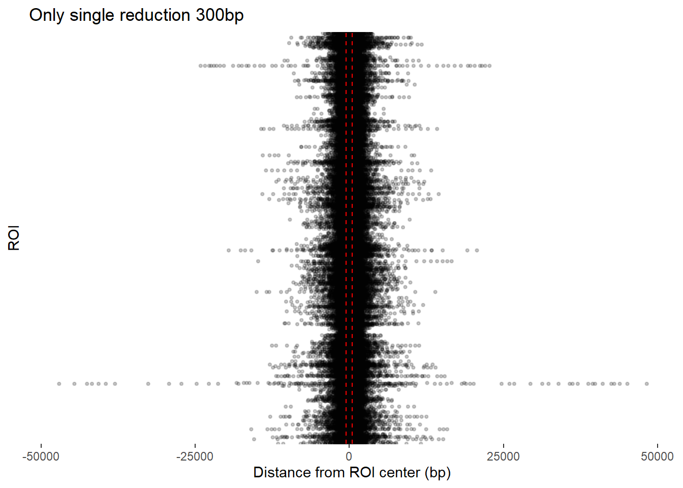
sessionInfo()R version 4.4.2 (2024-10-31 ucrt)
Platform: x86_64-w64-mingw32/x64
Running under: Windows 11 x64 (build 26200)
Matrix products: default
locale:
[1] LC_COLLATE=English_United States.utf8
[2] LC_CTYPE=English_United States.utf8
[3] LC_MONETARY=English_United States.utf8
[4] LC_NUMERIC=C
[5] LC_TIME=English_United States.utf8
time zone: America/Chicago
tzcode source: internal
attached base packages:
[1] grid stats4 stats graphics grDevices utils datasets
[8] methods base
other attached packages:
[1] ChIPseeker_1.42.1 BiocParallel_1.40.2 rtracklayer_1.66.0
[4] genomation_1.38.0 plyranges_1.26.0 GenomicRanges_1.58.0
[7] GenomeInfoDb_1.42.3 IRanges_2.40.1 S4Vectors_0.44.0
[10] BiocGenerics_0.52.0 lubridate_1.9.4 forcats_1.0.0
[13] stringr_1.5.1 dplyr_1.1.4 purrr_1.1.0
[16] readr_2.1.5 tidyr_1.3.1 tibble_3.3.0
[19] ggplot2_3.5.2 tidyverse_2.0.0 workflowr_1.7.1
loaded via a namespace (and not attached):
[1] RColorBrewer_1.1-3
[2] rstudioapi_0.17.1
[3] jsonlite_2.0.0
[4] magrittr_2.0.3
[5] ggbeeswarm_0.7.2
[6] ggtangle_0.0.7
[7] GenomicFeatures_1.58.0
[8] farver_2.1.2
[9] rmarkdown_2.29
[10] fs_1.6.6
[11] BiocIO_1.16.0
[12] zlibbioc_1.52.0
[13] vctrs_0.6.5
[14] Cairo_1.6-5
[15] memoise_2.0.1
[16] Rsamtools_2.22.0
[17] RCurl_1.98-1.17
[18] ggtree_3.14.0
[19] htmltools_0.5.8.1
[20] S4Arrays_1.6.0
[21] TxDb.Hsapiens.UCSC.hg19.knownGene_3.2.2
[22] plotrix_3.8-4
[23] curl_7.0.0
[24] SparseArray_1.6.2
[25] gridGraphics_0.5-1
[26] sass_0.4.10
[27] KernSmooth_2.23-26
[28] bslib_0.9.0
[29] plyr_1.8.9
[30] impute_1.80.0
[31] cachem_1.1.0
[32] GenomicAlignments_1.42.0
[33] igraph_2.1.4
[34] whisker_0.4.1
[35] lifecycle_1.0.4
[36] pkgconfig_2.0.3
[37] Matrix_1.7-3
[38] R6_2.6.1
[39] fastmap_1.2.0
[40] GenomeInfoDbData_1.2.13
[41] MatrixGenerics_1.18.1
[42] digest_0.6.37
[43] aplot_0.2.8
[44] enrichplot_1.26.6
[45] colorspace_2.1-1
[46] patchwork_1.3.2
[47] AnnotationDbi_1.68.0
[48] ps_1.9.1
[49] rprojroot_2.1.1
[50] RSQLite_2.4.3
[51] labeling_0.4.3
[52] timechange_0.3.0
[53] mgcv_1.9-3
[54] httr_1.4.7
[55] abind_1.4-8
[56] compiler_4.4.2
[57] bit64_4.6.0-1
[58] withr_3.0.2
[59] DBI_1.2.3
[60] gplots_3.2.0
[61] R.utils_2.13.0
[62] rappdirs_0.3.3
[63] DelayedArray_0.32.0
[64] rjson_0.2.23
[65] caTools_1.18.3
[66] gtools_3.9.5
[67] tools_4.4.2
[68] vipor_0.4.7
[69] beeswarm_0.4.0
[70] ape_5.8-1
[71] httpuv_1.6.16
[72] R.oo_1.27.1
[73] glue_1.8.0
[74] restfulr_0.0.16
[75] callr_3.7.6
[76] nlme_3.1-168
[77] GOSemSim_2.32.0
[78] promises_1.3.3
[79] getPass_0.2-4
[80] gridBase_0.4-7
[81] reshape2_1.4.4
[82] snow_0.4-4
[83] fgsea_1.32.4
[84] generics_0.1.4
[85] gtable_0.3.6
[86] BSgenome_1.74.0
[87] tzdb_0.5.0
[88] R.methodsS3_1.8.2
[89] seqPattern_1.38.0
[90] data.table_1.17.8
[91] hms_1.1.3
[92] XVector_0.46.0
[93] ggrepel_0.9.6
[94] pillar_1.11.0
[95] yulab.utils_0.2.1
[96] vroom_1.6.5
[97] later_1.4.2
[98] splines_4.4.2
[99] treeio_1.30.0
[100] lattice_0.22-7
[101] bit_4.6.0
[102] tidyselect_1.2.1
[103] GO.db_3.20.0
[104] Biostrings_2.74.1
[105] knitr_1.50
[106] git2r_0.36.2
[107] SummarizedExperiment_1.36.0
[108] xfun_0.52
[109] Biobase_2.66.0
[110] matrixStats_1.5.0
[111] stringi_1.8.7
[112] UCSC.utils_1.2.0
[113] lazyeval_0.2.2
[114] ggfun_0.2.0
[115] yaml_2.3.10
[116] boot_1.3-32
[117] evaluate_1.0.5
[118] codetools_0.2-20
[119] qvalue_2.38.0
[120] ggplotify_0.1.2
[121] cli_3.6.5
[122] processx_3.8.6
[123] jquerylib_0.1.4
[124] dichromat_2.0-0.1
[125] Rcpp_1.1.0
[126] png_0.1-8
[127] ggrastr_1.0.2
[128] XML_3.99-0.18
[129] parallel_4.4.2
[130] blob_1.2.4
[131] DOSE_4.0.1
[132] bitops_1.0-9
[133] viridisLite_0.4.2
[134] tidytree_0.4.6
[135] scales_1.4.0
[136] crayon_1.5.3
[137] rlang_1.1.6
[138] fastmatch_1.1-6
[139] cowplot_1.2.0
[140] KEGGREST_1.46.0