Characterise Simulation Data
Ross Gayler
2021-06-22
Last updated: 2021-07-02
Checks: 7 0
Knit directory:
VSA_altitude_hold/
This reproducible R Markdown analysis was created with workflowr (version 1.6.2). The Checks tab describes the reproducibility checks that were applied when the results were created. The Past versions tab lists the development history.
Great! Since the R Markdown file has been committed to the Git repository, you know the exact version of the code that produced these results.
Great job! The global environment was empty. Objects defined in the global environment can affect the analysis in your R Markdown file in unknown ways. For reproduciblity it’s best to always run the code in an empty environment.
The command set.seed(20210617) was run prior to running the code in the R Markdown file.
Setting a seed ensures that any results that rely on randomness, e.g.
subsampling or permutations, are reproducible.
Great job! Recording the operating system, R version, and package versions is critical for reproducibility.
Nice! There were no cached chunks for this analysis, so you can be confident that you successfully produced the results during this run.
Great job! Using relative paths to the files within your workflowr project makes it easier to run your code on other machines.
Great! You are using Git for version control. Tracking code development and connecting the code version to the results is critical for reproducibility.
The results in this page were generated with repository version b525eff. See the Past versions tab to see a history of the changes made to the R Markdown and HTML files.
Note that you need to be careful to ensure that all relevant files for the
analysis have been committed to Git prior to generating the results (you can
use wflow_publish or wflow_git_commit). workflowr only
checks the R Markdown file, but you know if there are other scripts or data
files that it depends on. Below is the status of the Git repository when the
results were generated:
Ignored files:
    Ignored:    .Rhistory
    Ignored:    .Rproj.user/
    Ignored:    renv/library/
    Ignored:    renv/staging/

Unstaged changes:
    Modified:   renv.lock
Note that any generated files, e.g. HTML, png, CSS, etc., are not included in this status report because it is ok for generated content to have uncommitted changes.
These are the previous versions of the repository in which changes were made
to the R Markdown (analysis/characterise_data.Rmd) and HTML (docs/characterise_data.html)
files. If you’ve configured a remote Git repository (see
?wflow_git_remote), click on the hyperlinks in the table below to
view the files as they were in that past version.
| File | Version | Author | Date | Message |
|---|---|---|---|---|
| Rmd | 3b6288c | Ross Gayler | 2021-06-30 | WIP |
| html | 3b6288c | Ross Gayler | 2021-06-30 | WIP |
| Rmd | 7eae4c3 | Ross Gayler | 2021-06-26 | Check simulation data: initial values and z versus dz |
| html | 7eae4c3 | Ross Gayler | 2021-06-26 | Check simulation data: initial values and z versus dz |
| Rmd | c39cb39 | Ross Gayler | 2021-06-25 | Take first look at simulation data |
| html | c39cb39 | Ross Gayler | 2021-06-25 | Take first look at simulation data |
This notebook characterises data generated by the simulation of the classically implemented altitude hold controller. We need to understand the properties of the signals in order to design VSA implementations of them.
The values to be characterised are all the real scalars corresponding to the nodes in the data flow diagram for Design 01.
1 Data
The data is generated from runs of the classically implemented simulation.
The data files are stored in the data directory.
The data is supplied as CSV files, each file corresponding to a different run of the simulation.
Each run of the simulation corresponds to a set of starting conditions and parameters.
The only starting condition that varies between runs is the initial altitude. In effect, the multicopter is dropped from some height, with the motors stopped and the drone must command the motors to attain the target altitude.
The name of each data file contains the values of all the parameters. In this work the target altitude is always constant at 5 metres, but more generally this should be treated as a demand which can vary with time.
Each row of the data file corresponds to a point in time and successive rows correspond to successive points in time. (This is a discrete time simulation with fixed time steps.)
Each file contains 500 time steps.
Each columns of the data file corresponds to a node of the data flow diagram.
Only a subset of the nodes are supplied (the nodes in rectangular boxes in the DFD supplied by Simon Levy) and the values of the other nodes can be reconstructed mathematically.
The values supplied from the input files are recorded to three decimal places, so there is scope for approximation error due to the limited precision.
Where a node value is supplied from the input file use that value and can also be mathematically reconstructed from upstream values, us the input value (rather than the reconstructed value) as input to downstream calculations. This is to avoid propagating approximation errors.
1.1 Read data
Read the data from the simulations and mathematically reconstruct the values of the nodes not included in the input files.
# function to clip value to a range
clip <- function(
  x, # numeric
  x_min, # numeric[1] - minimum output value
  x_max  # numeric[1] - maximum output value
) # value # numeric - x constrained to the range [x_min, x_max]
  {
  x %>% pmax(x_min) %>% pmin(x_max)
}

# function to extract a numeric parameter value from the file name
get_param_num <- function(
  file, # character - vector of file names
  regexp # character[1] - regular expression for "param=value"
         # use a capture group to get the value part
) # value # numeric - vector of parameter values
{
  file %>% str_match(regexp) %>%
      subset(select = 2) %>% as.numeric()
}

# function to extract a logical parameter value from the file name
get_param_log <- function(
  file, # character - vector of file names
  regexp # character[1] - regular expression for "param=value"
  # use a capture group to get the value part
  # value *must* be T or F
) # value # logical - vector of logical parameter values
{
  file %>% str_match(regexp) %>%
    subset(select = 2) %>% as.character() %>% "=="("T")
}

# read the data
d_wide <- fs::dir_ls(path = here::here("data"), regexp = "/k_start=.*\\.csv$") %>% # get file paths
  vroom::vroom(id = "file") %>% # read files
  dplyr::mutate( # add extra columns
    file = file %>% fs::path_ext_remove() %>% fs::path_file(), # get file name
    # get parameters
    k_start  = file %>% get_param_num("k_start=([.0-9]+)"),
    k_p      = file %>% get_param_num("kp=([.0-9]+)"),
    k_i      = file %>% get_param_num("Ki=([.0-9]+)"),
    k_tgt    = file %>% get_param_num("k_tgt=([.0-9]+)"),
    k_windup = file %>% get_param_num("k_windup=([.0-9]+)"),
    uclip    = file %>% get_param_log("_uclip=([TF])"),
    dz0      = file %>% get_param_log("_dz0=([TF])"),
    # reconstruct the missing nodes
    i1 = k_tgt - z,
    i2 = i1 - dz,
    i3 = e * k_p,
    i9 = lag(ei, n = 1, default = 0),
    i4 = e + i9,
    i5 = i4 %>% clip(-k_windup, k_windup),
    i6 = ei * k_i,
    i7 = i3 + i6,
    i8 = i7 %>% clip(0, 1)
  ) %>%
  # add time variable per file
  dplyr::group_by(file) %>%
  dplyr::mutate(t = 1:n()) %>%
  dplyr::ungroup()
Rows: 3500 Columns: 6── Column specification ────────────────────────────────────────────────────────
Delimiter: ","
dbl (5): z, dz, e, ei, u
ℹ Use `spec()` to retrieve the full column specification for this data.
ℹ Specify the column types or set `show_col_types = FALSE` to quiet this message.dplyr::glimpse(d_wide)Rows: 3,500
Columns: 23
$ file <chr> "k_start=10.00_k_tgt=5.00_kp=0.20_Ki=3.00_k_windup=0.20_uclip…
$ z <dbl> 10.000, 9.999, 9.998, 9.995, 9.992, 9.987, 9.982, 9.975, 9.96…
$ dz <dbl> -0.058, -0.156, -0.254, -0.352, -0.450, -0.548, -0.646, -0.74…
$ e <dbl> -4.942, -4.843, -4.744, -4.643, -4.542, -4.439, -4.335, -4.23…
$ ei <dbl> -0.2, -0.2, -0.2, -0.2, -0.2, -0.2, -0.2, -0.2, -0.2, -0.2, -…
$ u <dbl> 0, 0, 0, 0, 0, 0, 0, 0, 0, 0, 0, 0, 0, 0, 0, 0, 0, 0, 0, 0, 0…
$ k_start <dbl> 10, 10, 10, 10, 10, 10, 10, 10, 10, 10, 10, 10, 10, 10, 10, 1…
$ k_p <dbl> 0.2, 0.2, 0.2, 0.2, 0.2, 0.2, 0.2, 0.2, 0.2, 0.2, 0.2, 0.2, 0…
$ k_i <dbl> 3, 3, 3, 3, 3, 3, 3, 3, 3, 3, 3, 3, 3, 3, 3, 3, 3, 3, 3, 3, 3…
$ k_tgt <dbl> 5, 5, 5, 5, 5, 5, 5, 5, 5, 5, 5, 5, 5, 5, 5, 5, 5, 5, 5, 5, 5…
$ k_windup <dbl> 0.2, 0.2, 0.2, 0.2, 0.2, 0.2, 0.2, 0.2, 0.2, 0.2, 0.2, 0.2, 0…
$ uclip <lgl> TRUE, TRUE, TRUE, TRUE, TRUE, TRUE, TRUE, TRUE, TRUE, TRUE, T…
$ dz0 <lgl> FALSE, FALSE, FALSE, FALSE, FALSE, FALSE, FALSE, FALSE, FALSE…
$ i1 <dbl> -5.000, -4.999, -4.998, -4.995, -4.992, -4.987, -4.982, -4.97…
$ i2 <dbl> -4.942, -4.843, -4.744, -4.643, -4.542, -4.439, -4.336, -4.23…
$ i3 <dbl> -0.9884, -0.9686, -0.9488, -0.9286, -0.9084, -0.8878, -0.8670…
$ i9 <dbl> 0.0, -0.2, -0.2, -0.2, -0.2, -0.2, -0.2, -0.2, -0.2, -0.2, -0…
$ i4 <dbl> -4.942, -5.043, -4.944, -4.843, -4.742, -4.639, -4.535, -4.43…
$ i5 <dbl> -0.2, -0.2, -0.2, -0.2, -0.2, -0.2, -0.2, -0.2, -0.2, -0.2, -…
$ i6 <dbl> -0.6, -0.6, -0.6, -0.6, -0.6, -0.6, -0.6, -0.6, -0.6, -0.6, -…
$ i7 <dbl> -1.5884, -1.5686, -1.5488, -1.5286, -1.5084, -1.4878, -1.4670…
$ i8 <dbl> 0, 0, 0, 0, 0, 0, 0, 0, 0, 0, 0, 0, 0, 0, 0, 0, 0, 0, 0, 0, 0…
$ t <int> 1, 2, 3, 4, 5, 6, 7, 8, 9, 10, 11, 12, 13, 14, 15, 16, 17, 18…1.2 Check data
Check the data for consistency.
1.2.1 Initial values
The different starting conditions correspond to the multicopter being dropped/released at different altitudes. At the moment of release the multicopter should be at exactly the starting altitude and have zero vertical velocity. Check that this is true.
- The initial vertical velocities (\(dz\)) are nonzero. The most likely interpretation is that the \(z\) and \(dz\) values are skewed by one time step. An alternative interpretation is that the multicopter was released one time step earlier and a little higher than the target altitude so that it passes through the target altitude exactly one time step after release.
This apparent skew probably doesn’t make any substantial difference to the qualitative performance of the system. However, it makes some of the graphs messier because the trajectory doesn’t start at zero. It may also lead to the altitude converging slightly off the target altitude because the “perceived” altitude is not quite time-aligned with the error signal.
1.2.2 Check \(z\) and \(dz\)
The altitude (\(z\)) and vertical velocity (\(dz\)) are input values fro the simulation data files. Given only a single point in time, they are independent variables. However, we are given a time series of values and the vertical velocity should be a function of the time series of altitude.
Given that the multicopter simulation is a discrete time simulation, the most likely interpretation is that \(dz\) is calculated as the difference between successive \(z\) values. Check whether that is the case.
Warning: Removed 7 rows containing missing values (geom_point).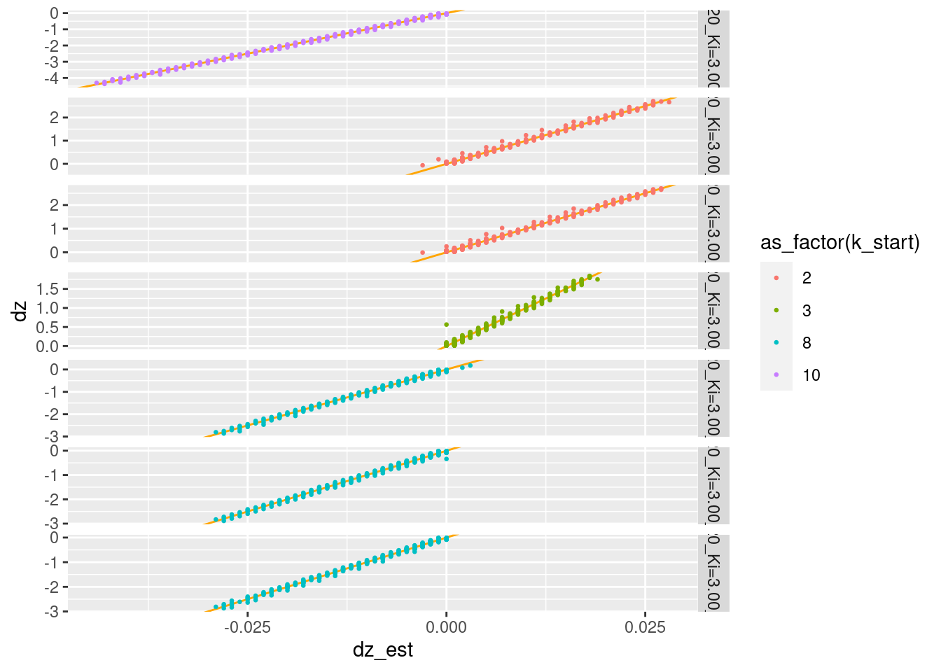
The supplied \(dz\) is a linear transform of estimated vertical velocity (difference between successive altitude values).
- I am prepared to believe that the inacurracy is due to the low precision of the values in the files.
But, the scaling is very different: \(dz = 100 dz_{est}\). The time step is 10 ms, so it looks like like \(dz\) is in units of metres per second and \(dz_{est}\) is in units of metres per time step.
Looking at the PID calculation of error (\(e\)): \[
\begin{aligned}
e &= k_{tgt} - z - dz \\
&= k_{tgt} - (z + dz)
\end{aligned}
\]
The term \((z + dz)\) is effectively a prediction of the altitude at the
next time step based on the altitude \(z\) and vertical velocity \(dz\) at
the previous time step. Thus, the error \(e\) is the difference between
the target altitude and the predicted altitude. This requires \(z\) and
\(dz\) to be measured in compatible units for the prediction \((z + dz)\) to
make sense. Both quantities must be measured in metres and \(dz\) must be
metres over the relevant time period, which is one time step.
Consequently, I believe \(dz\) is scaled wrongly because the prediction \((z + dz)\) is the prediction for a point 100 time steps in the future.
1.2.3 Check calculated values
Where possible compare the calculated values with the values recorded from the simulator.
Nodes with a single input edge can be checked against the output of the predecessor node.
The nodes which can be checked are: e, ei, u
- The reconstructed values which can be checked against values from the simulation are correct except for approximation error due to the low precision of the numbers in the files.
2 Distribution summary
Display a quick summary of the distributions of values of all the nodes.
Note that these summaries are over all the input files pooled.
| Name | d_wide |
| Number of rows | 3500 |
| Number of columns | 23 |
| _______________________ | |
| Column type frequency: | |
| character | 1 |
| logical | 2 |
| numeric | 20 |
| ________________________ | |
| Group variables | None |
Variable type: character
| skim_variable | n_missing | complete_rate | min | max | empty | n_unique | whitespace |
|---|---|---|---|---|---|---|---|
| file | 0 | 1 | 67 | 68 | 0 | 7 | 0 |
Variable type: logical
| skim_variable | n_missing | complete_rate | mean | count |
|---|---|---|---|---|
| uclip | 0 | 1 | 0.43 | FAL: 2000, TRU: 1500 |
| dz0 | 0 | 1 | 0.29 | FAL: 2500, TRU: 1000 |
Variable type: numeric
| skim_variable | n_missing | complete_rate | mean | sd | p0 | p25 | p50 | p75 | p100 | hist |
|---|---|---|---|---|---|---|---|---|---|---|
| z | 0 | 1 | 5.22 | 1.15 | 2.00 | 4.85 | 5.05 | 5.44 | 10.00 | ▁▇▃▁▁ |
| dz | 0 | 1 | -0.17 | 0.98 | -4.37 | -0.43 | -0.05 | 0.15 | 2.71 | ▁▁▅▇▁ |
| e | 0 | 1 | -0.05 | 0.46 | -4.94 | 0.00 | 0.00 | 0.00 | 3.32 | ▁▁▇▁▁ |
| ei | 0 | 1 | 0.16 | 0.07 | -0.20 | 0.17 | 0.17 | 0.18 | 0.20 | ▁▁▁▁▇ |
| u | 0 | 1 | 0.50 | 0.20 | -1.25 | 0.52 | 0.52 | 0.53 | 1.26 | ▁▁▁▇▁ |
| k_start | 0 | 1 | 5.86 | 3.14 | 2.00 | 2.00 | 8.00 | 8.00 | 10.00 | ▇▁▁▇▂ |
| k_p | 0 | 1 | 0.20 | 0.00 | 0.20 | 0.20 | 0.20 | 0.20 | 0.20 | ▁▁▇▁▁ |
| k_i | 0 | 1 | 3.00 | 0.00 | 3.00 | 3.00 | 3.00 | 3.00 | 3.00 | ▁▁▇▁▁ |
| k_tgt | 0 | 1 | 5.00 | 0.00 | 5.00 | 5.00 | 5.00 | 5.00 | 5.00 | ▁▁▇▁▁ |
| k_windup | 0 | 1 | 0.20 | 0.00 | 0.20 | 0.20 | 0.20 | 0.20 | 0.20 | ▁▁▇▁▁ |
| i1 | 0 | 1 | -0.22 | 1.15 | -5.00 | -0.44 | -0.05 | 0.15 | 3.00 | ▁▁▃▇▁ |
| i2 | 0 | 1 | -0.05 | 0.46 | -4.94 | 0.00 | 0.00 | 0.00 | 3.32 | ▁▁▇▁▁ |
| i3 | 0 | 1 | -0.01 | 0.09 | -0.99 | 0.00 | 0.00 | 0.00 | 0.66 | ▁▁▇▁▁ |
| i9 | 0 | 1 | 0.16 | 0.07 | -0.20 | 0.17 | 0.17 | 0.18 | 0.20 | ▁▁▁▁▇ |
| i4 | 0 | 1 | 0.12 | 0.52 | -5.04 | 0.17 | 0.17 | 0.18 | 3.50 | ▁▁▁▇▁ |
| i5 | 0 | 1 | 0.16 | 0.07 | -0.20 | 0.17 | 0.17 | 0.18 | 0.20 | ▁▁▁▁▇ |
| i6 | 0 | 1 | 0.49 | 0.21 | -0.60 | 0.52 | 0.52 | 0.53 | 0.60 | ▁▁▁▁▇ |
| i7 | 0 | 1 | 0.48 | 0.29 | -1.59 | 0.52 | 0.52 | 0.53 | 1.26 | ▁▁▁▇▁ |
| i8 | 0 | 1 | 0.51 | 0.11 | 0.00 | 0.52 | 0.52 | 0.53 | 1.00 | ▁▁▇▁▁ |
| t | 0 | 1 | 250.50 | 144.36 | 1.00 | 125.75 | 250.50 | 375.25 | 500.00 | ▇▇▇▇▇ |
3 Plots
Plot the relationships between the major nodes. This is not necessarily of immediate use in deciding the design fo VSA components, but gives a feel for the dynamics of the system.
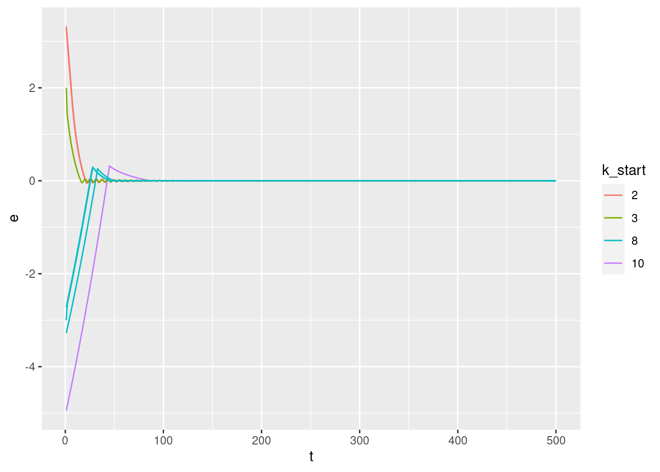
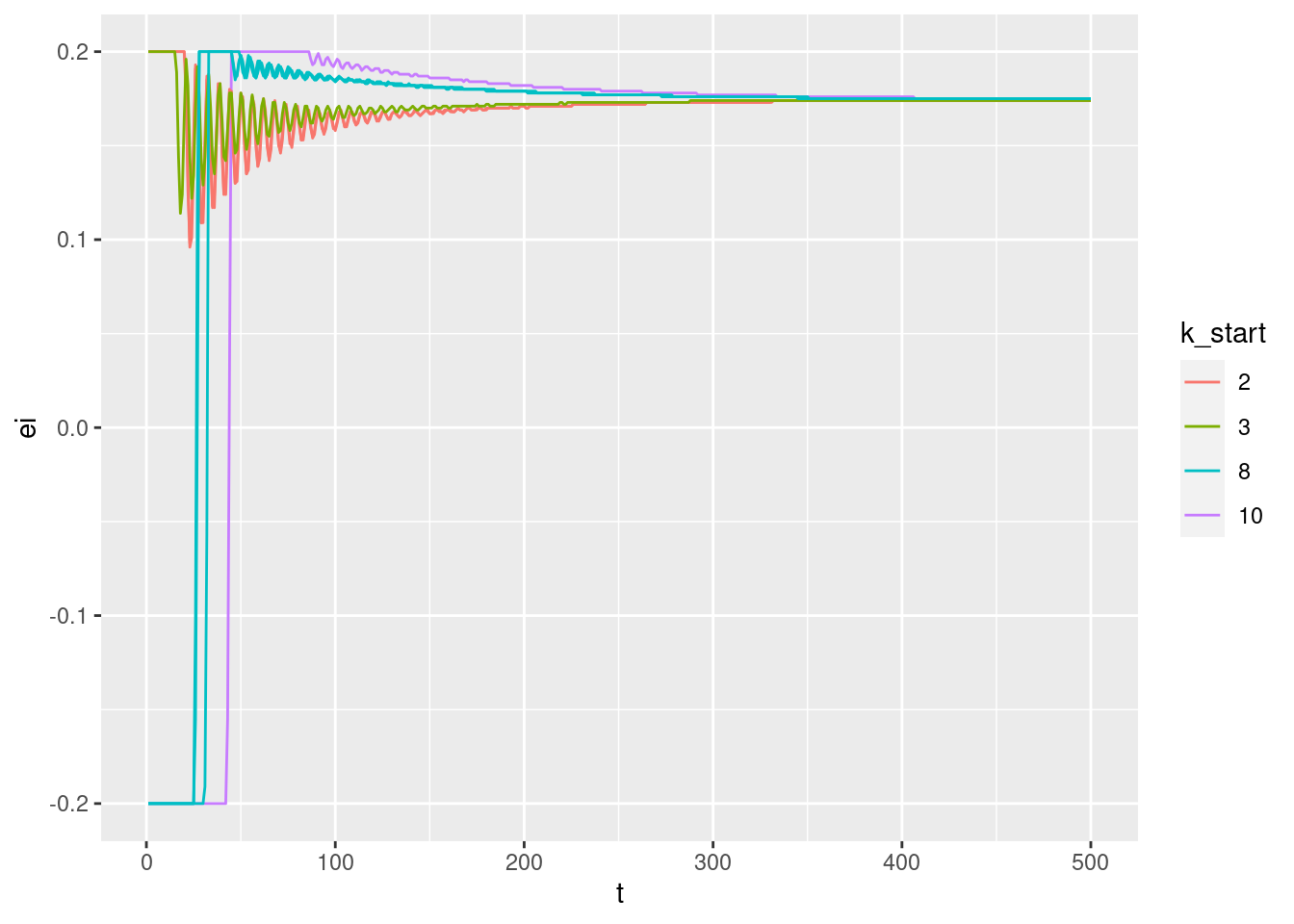
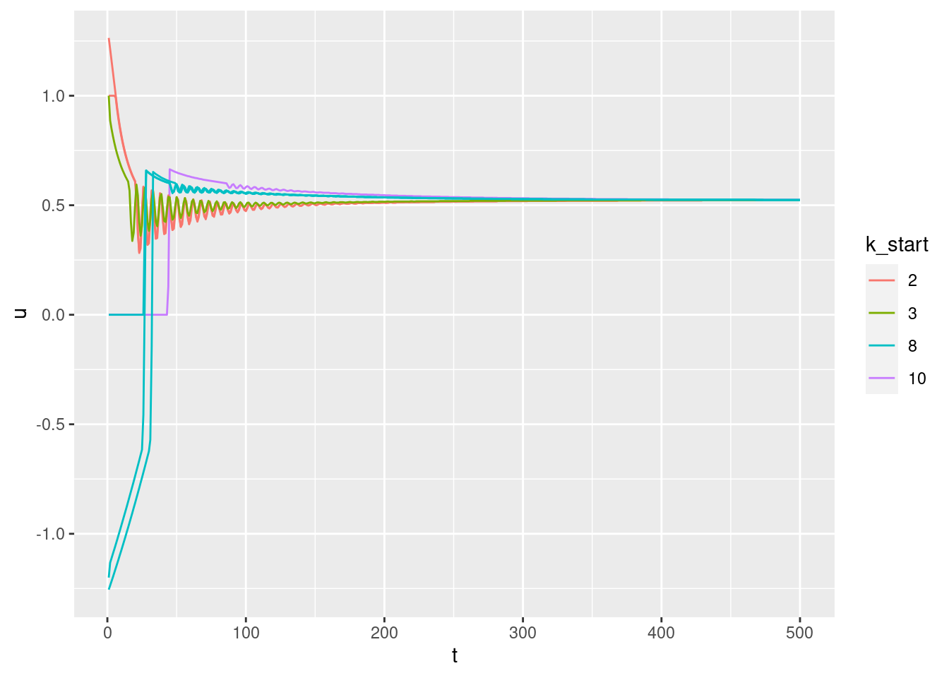
3.1 Time explicit
Show the values of the major nodes as a function of time.
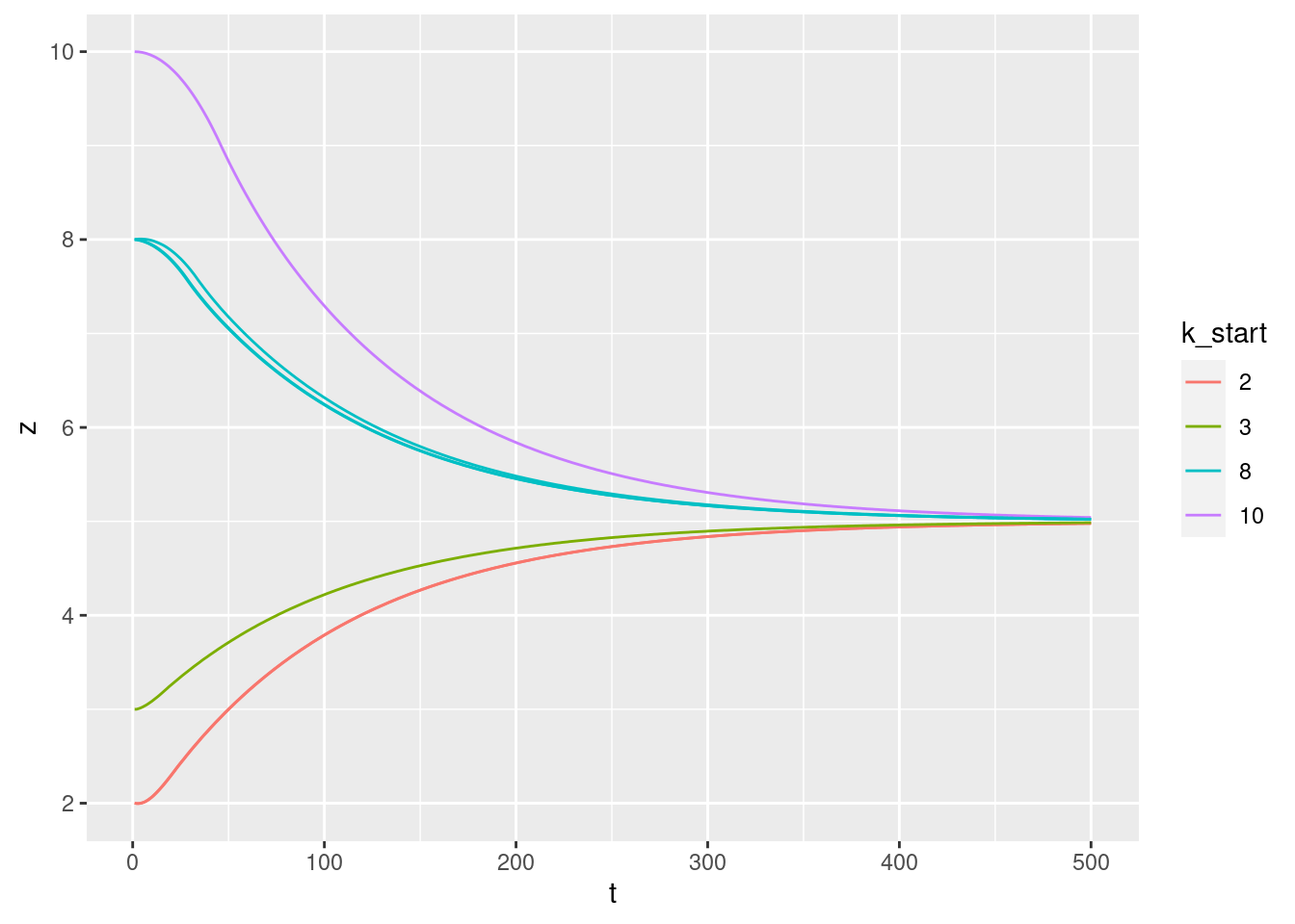
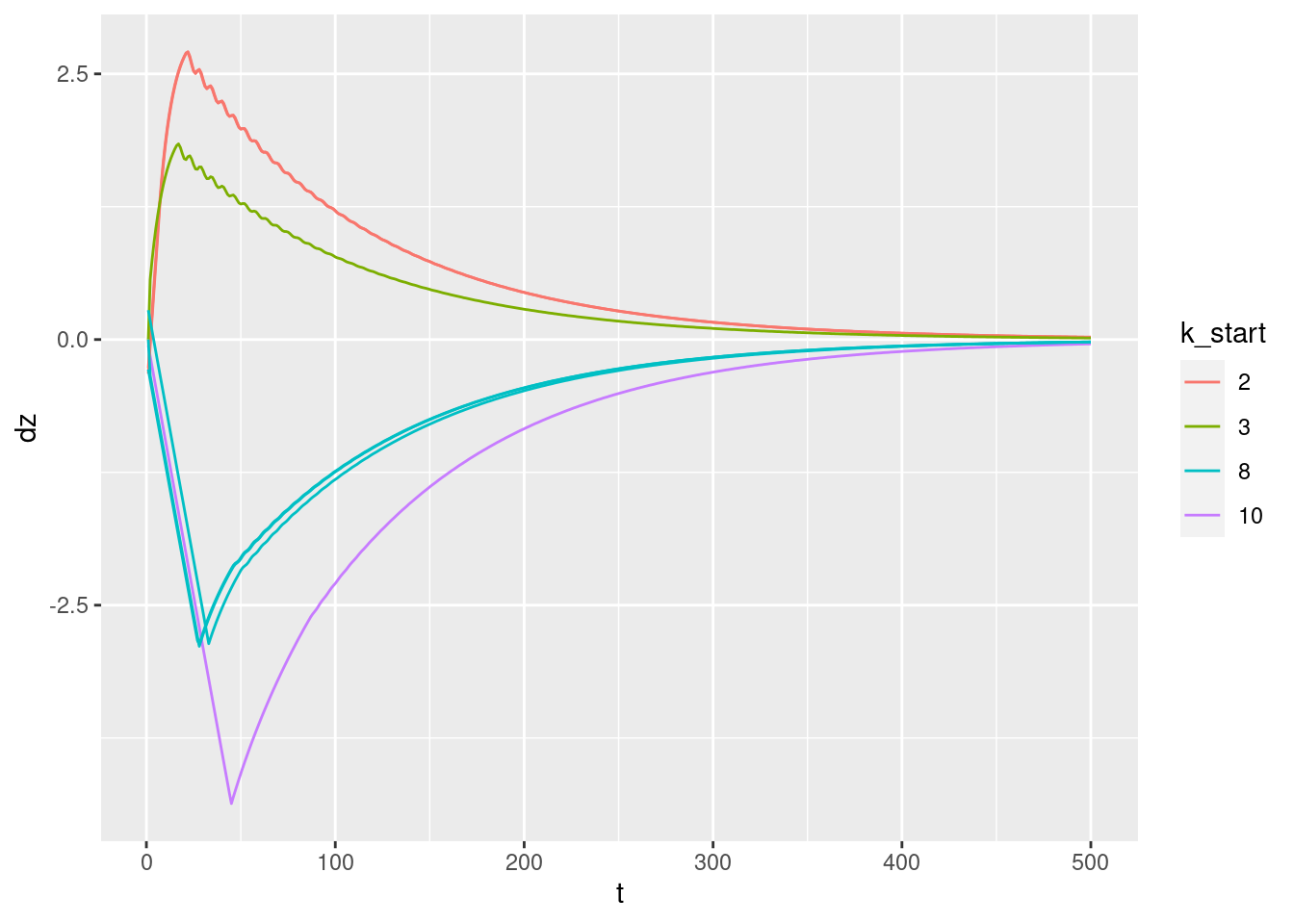
Warning: Removed 1 row(s) containing missing values (geom_path).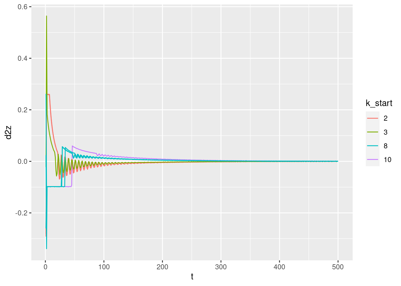
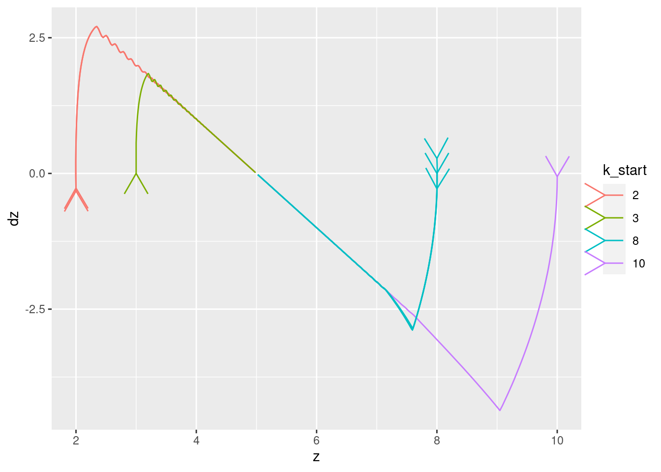
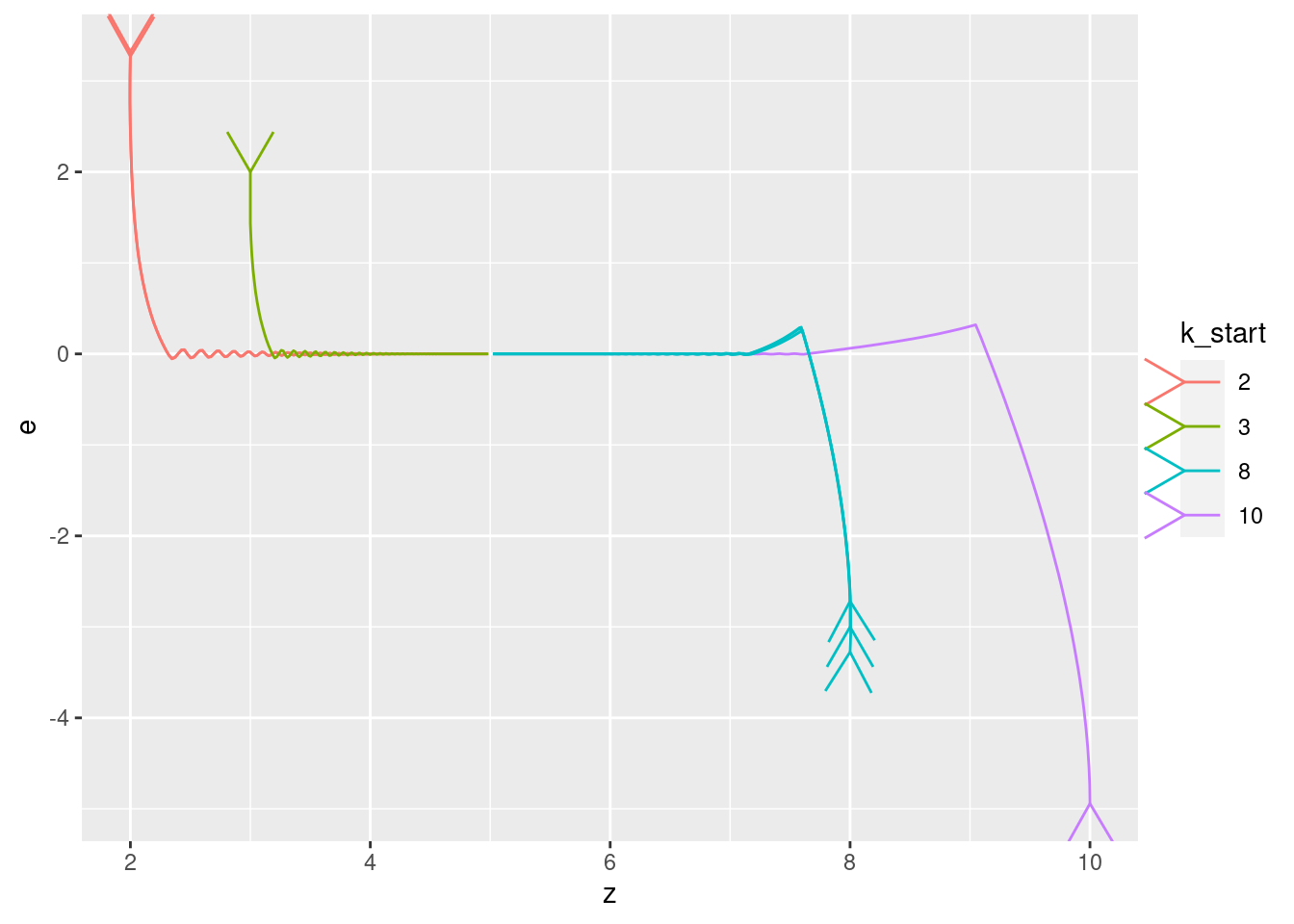
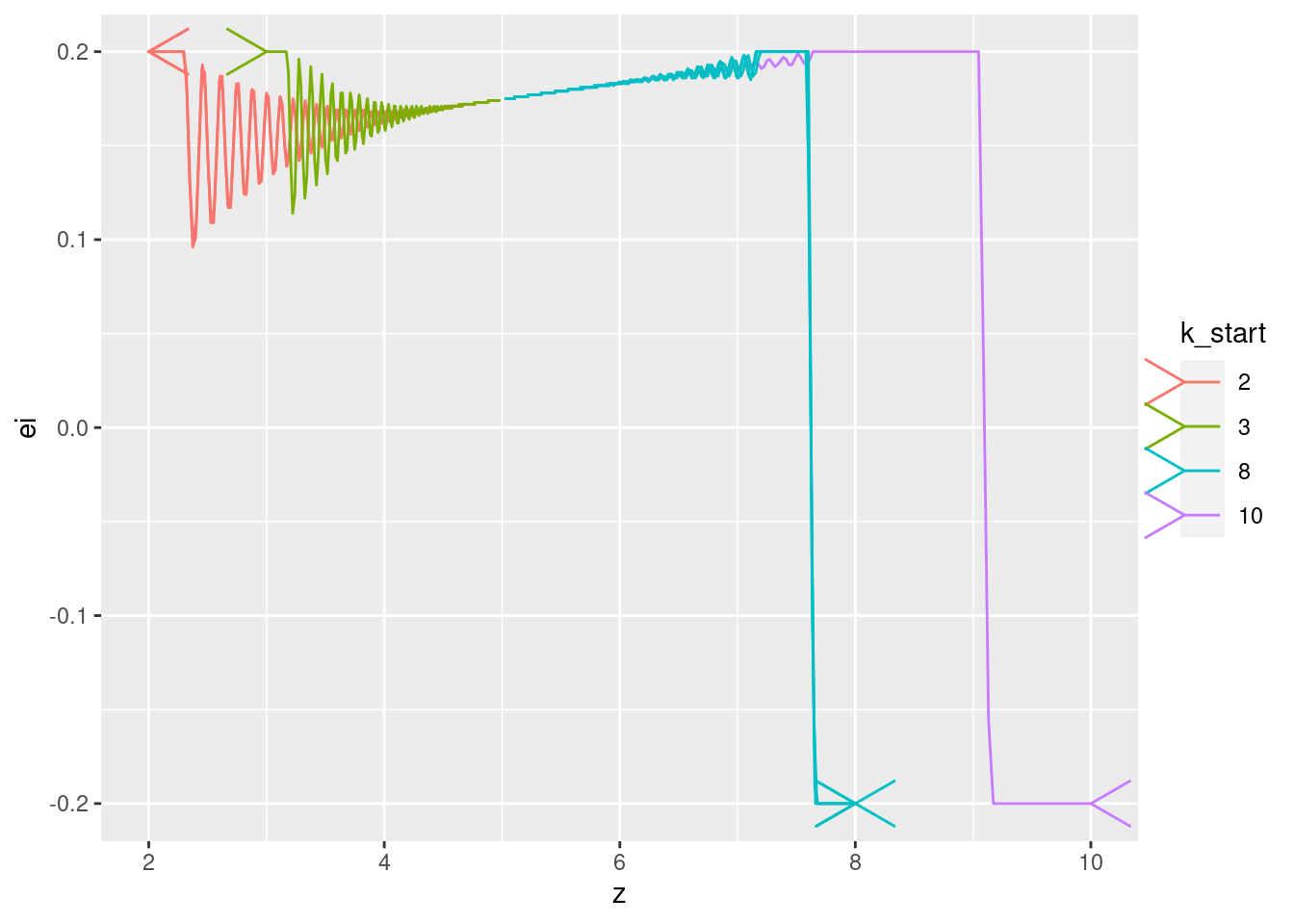
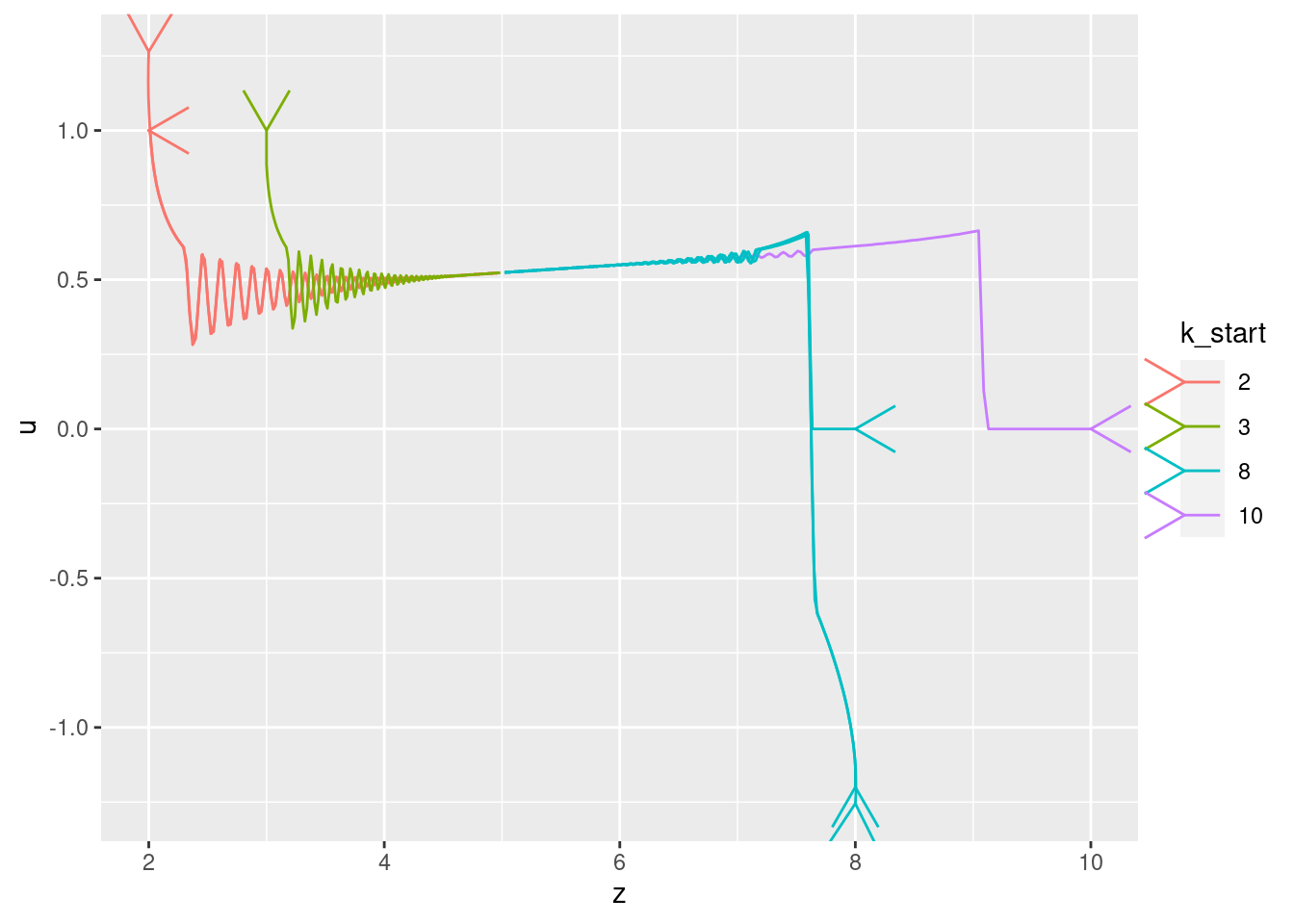
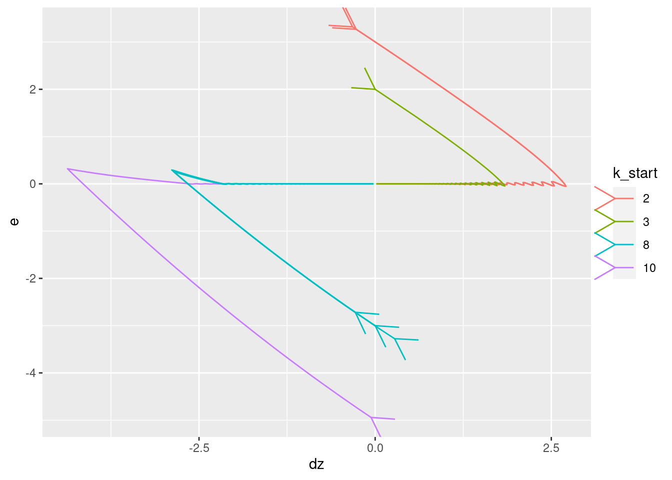
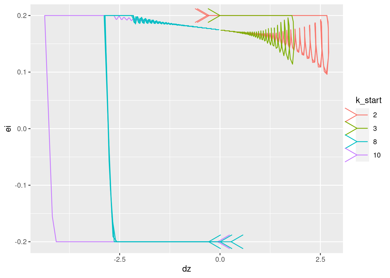
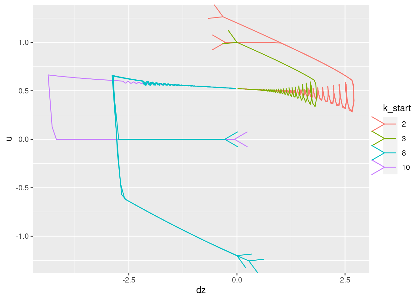
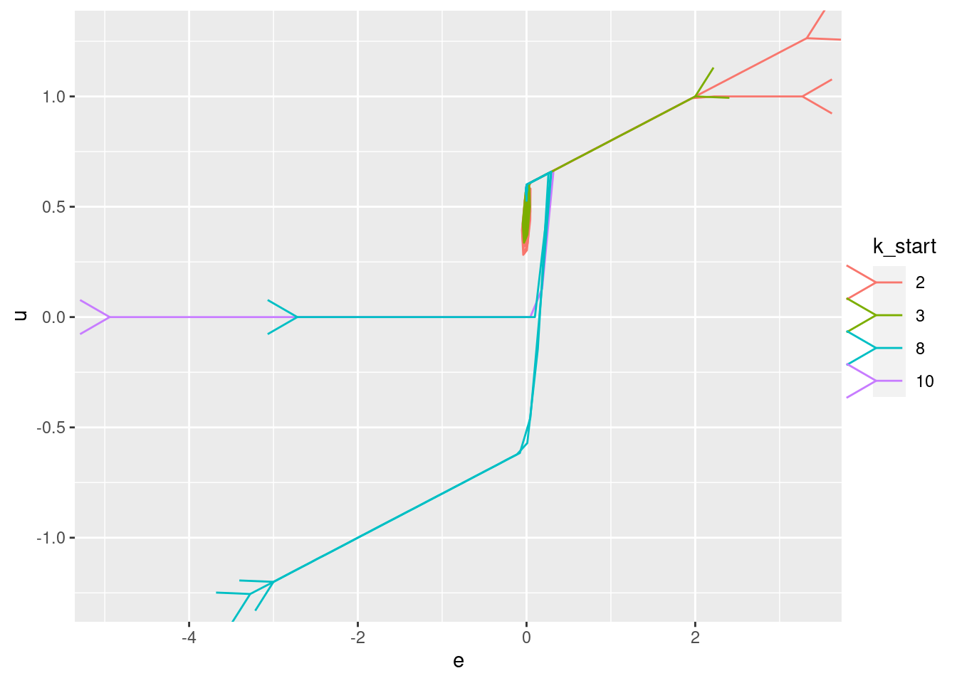
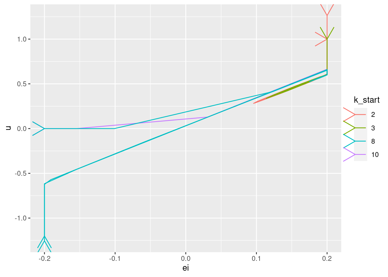
3.2 Time implicit
Show the values of the major nodes as a function of each other (with time implicit).
| Version | Author | Date |
|---|---|---|
| b525eff | Ross Gayler | 2021-06-30 |
Warning: Removed 1 row(s) containing missing values (geom_path).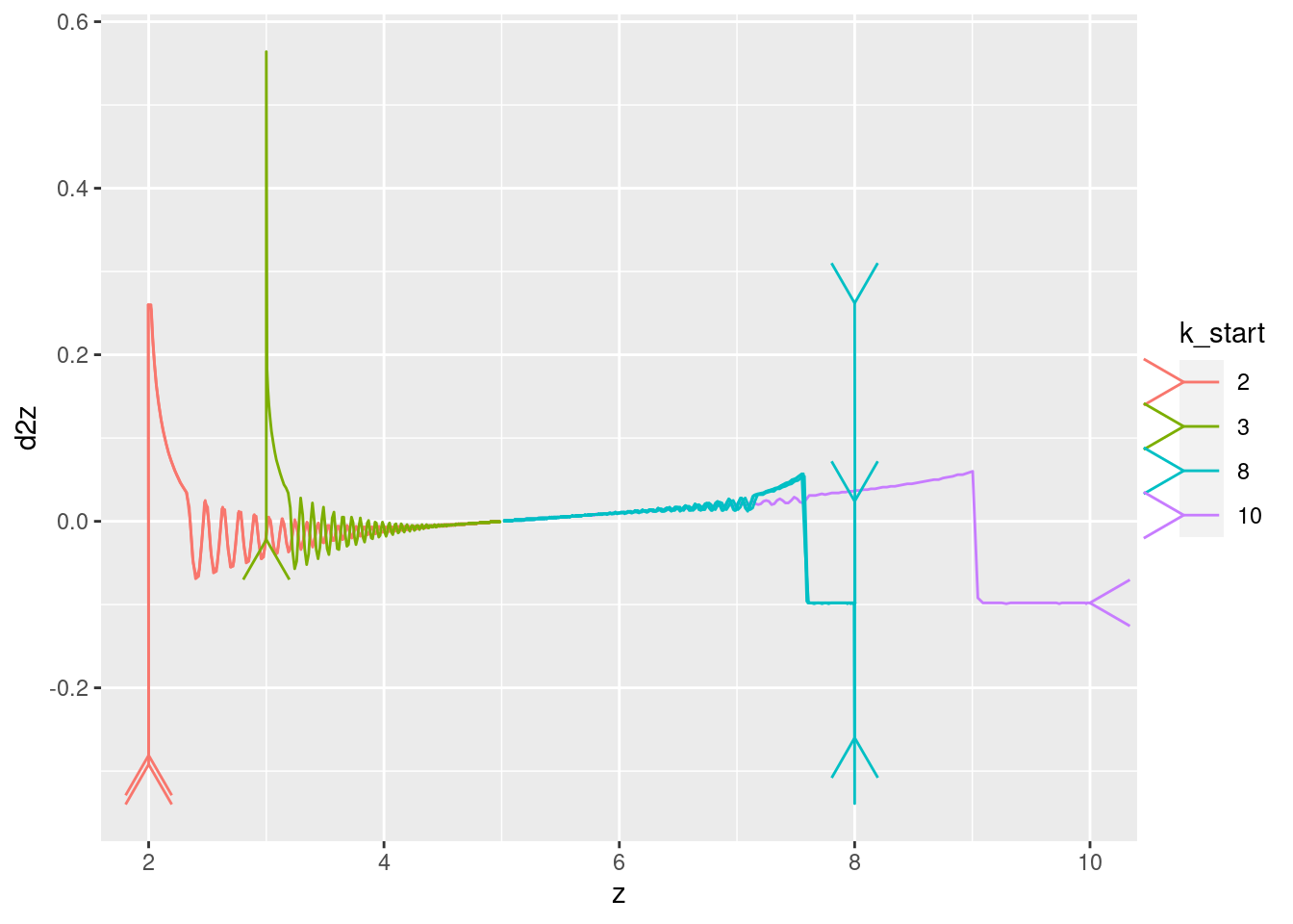
| Version | Author | Date |
|---|---|---|
| b525eff | Ross Gayler | 2021-06-30 |
| Version | Author | Date |
|---|---|---|
| b525eff | Ross Gayler | 2021-06-30 |
| Version | Author | Date |
|---|---|---|
| b525eff | Ross Gayler | 2021-06-30 |
| Version | Author | Date |
|---|---|---|
| b525eff | Ross Gayler | 2021-06-30 |
Warning: Removed 1 row(s) containing missing values (geom_path).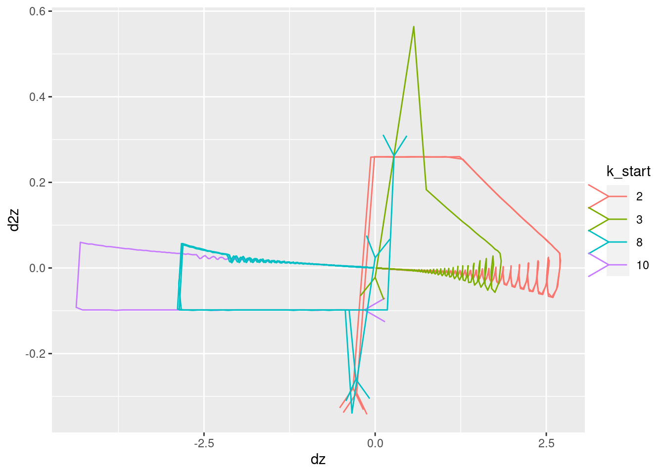
| Version | Author | Date |
|---|---|---|
| b525eff | Ross Gayler | 2021-06-30 |
| Version | Author | Date |
|---|---|---|
| b525eff | Ross Gayler | 2021-06-30 |
| Version | Author | Date |
|---|---|---|
| b525eff | Ross Gayler | 2021-06-30 |
| Version | Author | Date |
|---|---|---|
| b525eff | Ross Gayler | 2021-06-30 |
Warning: Removed 1 row(s) containing missing values (geom_path).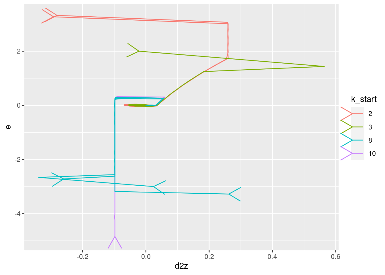
| Version | Author | Date |
|---|---|---|
| b525eff | Ross Gayler | 2021-06-30 |
Warning: Removed 1 row(s) containing missing values (geom_path).
| Version | Author | Date |
|---|---|---|
| b525eff | Ross Gayler | 2021-06-30 |
Warning: Removed 1 row(s) containing missing values (geom_path).
| Version | Author | Date |
|---|---|---|
| b525eff | Ross Gayler | 2021-06-30 |
| Version | Author | Date |
|---|---|---|
| b525eff | Ross Gayler | 2021-06-30 |
| Version | Author | Date |
|---|---|---|
| b525eff | Ross Gayler | 2021-06-30 |
| Version | Author | Date |
|---|---|---|
| b525eff | Ross Gayler | 2021-06-30 |
R version 4.1.0 (2021-05-18)
Platform: x86_64-pc-linux-gnu (64-bit)
Running under: Ubuntu 21.04

Matrix products: default
BLAS:   /usr/lib/x86_64-linux-gnu/blas/libblas.so.3.9.0
LAPACK: /usr/lib/x86_64-linux-gnu/lapack/liblapack.so.3.9.0

locale:
 [1] LC_CTYPE=en_AU.UTF-8       LC_NUMERIC=C
 [3] LC_TIME=en_AU.UTF-8        LC_COLLATE=en_AU.UTF-8
 [5] LC_MONETARY=en_AU.UTF-8    LC_MESSAGES=en_AU.UTF-8
 [7] LC_PAPER=en_AU.UTF-8       LC_NAME=C
 [9] LC_ADDRESS=C               LC_TELEPHONE=C
[11] LC_MEASUREMENT=en_AU.UTF-8 LC_IDENTIFICATION=C

attached base packages:
[1] stats     graphics  grDevices datasets  utils     methods   base

other attached packages:
[1] ggplot2_3.3.5 forcats_0.5.1 skimr_2.1.3   stringr_1.4.0 DT_0.18
[6] dplyr_1.0.7   vroom_1.5.1   here_1.0.1    fs_1.5.0

loaded via a namespace (and not attached):
 [1] tidyselect_1.1.1  xfun_0.24         repr_1.1.3        purrr_0.3.4
 [5] colorspace_2.0-2  vctrs_0.3.8       generics_0.1.0    htmltools_0.5.1.1
 [9] yaml_2.2.1        base64enc_0.1-3   utf8_1.2.1        rlang_0.4.11
[13] later_1.2.0       pillar_1.6.1      glue_1.4.2        withr_2.4.2
[17] bit64_4.0.5       lifecycle_1.0.0   munsell_0.5.0     gtable_0.3.0
[21] workflowr_1.6.2   htmlwidgets_1.5.3 evaluate_0.14     labeling_0.4.2
[25] knitr_1.33        tzdb_0.1.1        crosstalk_1.1.1   httpuv_1.6.1
[29] parallel_4.1.0    fansi_0.5.0       highr_0.9         Rcpp_1.0.6
[33] renv_0.13.2       promises_1.2.0.1  scales_1.1.1      jsonlite_1.7.2
[37] farver_2.1.0      bit_4.0.4         digest_0.6.27     stringi_1.6.2
[41] bookdown_0.22     rprojroot_2.0.2   grid_4.1.0        cli_3.0.0
[45] tools_4.1.0       magrittr_2.0.1    tibble_3.1.2      tidyr_1.1.3
[49] crayon_1.4.1      whisker_0.4       pkgconfig_2.0.3   ellipsis_0.3.2
[53] rmarkdown_2.9     rstudioapi_0.13   R6_2.5.0          git2r_0.28.0
[57] compiler_4.1.0