VSA Implementation of PID Task Analysis
Ross Gayler
2021-0
Last updated: 2021-09-12
Checks: 7 0
Knit directory:
VSA_altitude_hold/
This reproducible R Markdown analysis was created with workflowr (version 1.6.2). The Checks tab describes the reproducibility checks that were applied when the results were created. The Past versions tab lists the development history.
Great! Since the R Markdown file has been committed to the Git repository, you know the exact version of the code that produced these results.
Great job! The global environment was empty. Objects defined in the global environment can affect the analysis in your R Markdown file in unknown ways. For reproduciblity it’s best to always run the code in an empty environment.
The command set.seed(20210617) was run prior to running the code in the R Markdown file.
Setting a seed ensures that any results that rely on randomness, e.g.
subsampling or permutations, are reproducible.
Great job! Recording the operating system, R version, and package versions is critical for reproducibility.
Nice! There were no cached chunks for this analysis, so you can be confident that you successfully produced the results during this run.
Great job! Using relative paths to the files within your workflowr project makes it easier to run your code on other machines.
Great! You are using Git for version control. Tracking code development and connecting the code version to the results is critical for reproducibility.
The results in this page were generated with repository version bf544c6. See the Past versions tab to see a history of the changes made to the R Markdown and HTML files.
Note that you need to be careful to ensure that all relevant files for the
analysis have been committed to Git prior to generating the results (you can
use wflow_publish or wflow_git_commit). workflowr only
checks the R Markdown file, but you know if there are other scripts or data
files that it depends on. Below is the status of the Git repository when the
results were generated:
Ignored files:
    Ignored:    .Rhistory
    Ignored:    .Rproj.user/
    Ignored:    renv/library/
    Ignored:    renv/local/
    Ignored:    renv/staging/
Note that any generated files, e.g. HTML, png, CSS, etc., are not included in this status report because it is ok for generated content to have uncommitted changes.
These are the previous versions of the repository in which changes were made
to the R Markdown (analysis/PID_task_analysis_VSA.Rmd) and HTML (docs/PID_task_analysis_VSA.html)
files. If you’ve configured a remote Git repository (see
?wflow_git_remote), click on the hyperlinks in the table below to
view the files as they were in that past version.
| File | Version | Author | Date | Message |
|---|---|---|---|---|
| Rmd | c51f761 | Ross Gayler | 2021-09-12 | WIP |
| html | c51f761 | Ross Gayler | 2021-09-12 | WIP |
| Rmd | da1f2fa | Ross Gayler | 2021-09-12 | WIP |
| html | da1f2fa | Ross Gayler | 2021-09-12 | WIP |
| Rmd | d27c378 | Ross Gayler | 2021-09-12 | WIP |
| html | d27c378 | Ross Gayler | 2021-09-12 | WIP |
| html | 2e83517 | Ross Gayler | 2021-09-11 | WIP |
| Rmd | ff213fa | Ross Gayler | 2021-09-11 | WIP |
| Rmd | 9a1cae9 | Ross Gayler | 2021-09-10 | WIP |
This notebook attempts to make a VSA implementation of the statistical model of the PID input/output function developed in the PID Task Analysis notebook.
The scalar inputs are represented using the spline encoding developed in the Linear Interpolation Spline notebook.
The VSA representations of the inputs are informed by the encodings developed in the feature engineering section.
The knots of the splines are chosen to allow curvature in the response surface where it is needed.
The input/output function will be learned by regression from the multi-target data set.
\(e\) and \(e_{orth}\) will be used as the input variables and I will ignore the VSA calculation of those quantities in this notebook.
We will build up the model incrementally to check that things are working as expected.
1 Read data
This notebook is based on the data generated by the simulation runs with multiple target altitudes per run.
Read the data from the simulations and mathematically reconstruct the values of the nodes not included in the input files.
Only a small subset of the nodes will be used in this notebook.
# function to clip value to a range
clip <- function(
  x, # numeric
  x_min, # numeric[1] - minimum output value
  x_max  # numeric[1] - maximum output value
) # value # numeric - x constrained to the range [x_min, x_max]
  {
  x %>% pmax(x_min) %>% pmin(x_max)
}

# function to extract a numeric parameter value from the file name
get_param_num <- function(
  file, # character - vector of file names
  regexp # character[1] - regular expression for "param=value"
         # use a capture group to get the value part
) # value # numeric - vector of parameter values
{
  file %>% str_match(regexp) %>%
      subset(select = 2) %>% as.numeric()
}

# function to extract a sequence of numeric parameter values from the file name
get_param_num_seq <- function(
  file, # character - vector of file names
  regexp # character[1] - regular expression for "param=value"
         # use a capture group to get the value part
) # value # character - character representation of a sequence, e.g. "(1,2,3)"
{
  file %>% str_match(regexp) %>%
      subset(select = 2) %>%
    str_replace_all(c("^" = "(", "_" = ",", "$" = ")")) # reformat as sequence
}

# function to extract a logical parameter value from the file name
get_param_log <- function(
  file, # character - vector of file names
  regexp # character[1] - regular expression for "param=value"
  # use a capture group to get the value part
  # value *must* be T or F
) # value # logical - vector of logical parameter values
{
  file %>% str_match(regexp) %>%
    subset(select = 2) %>% as.character() %>% "=="("T")
}

# read the data
d_wide <- fs::dir_ls(path = here::here("data", "multiple_target"), regexp = "/targets=.*\\.csv$") %>% # get file paths
  vroom::vroom(id = "file") %>% # read files
  dplyr::rename(k_tgt = target) %>% # rename for consistency with single target data
  dplyr::mutate( # add extra columns
    file = file %>% fs::path_ext_remove() %>% fs::path_file(), # get file name
    # get parameters
    targets  = file %>% get_param_num_seq("targets=([._0-9]+)_start="), # hacky
    k_start  = file %>% get_param_num("start=([.0-9]+)"),
    sim_id   = paste(targets, k_start), # short ID for each simulation
    k_p      = file %>% get_param_num("kp=([.0-9]+)"),
    k_i      = file %>% get_param_num("Ki=([.0-9]+)"),
    # k_tgt    = file %>% get_param_num("k_tgt=([.0-9]+)"), # no longer needed
    k_windup = file %>% get_param_num("k_windup=([.0-9]+)"),
    uclip    = FALSE, # constant across all files
    dz0      = TRUE, # constant across all files
    # Deal with the fact that the interpretation of the imported u value
    # depends on the uclip parameter
    u_import = u, # keep a copy of the imported value to one side
    u = dplyr::if_else(uclip, # make u the "correct" value
                       u_import,
                       clip(u_import, 0, 1)
                       ),
    # reconstruct the missing nodes
    i1 = k_tgt - z,
    i2 = i1 - dz,
    i3 = e * k_p,
    i9 = lag(ei, n = 1, default = 0), # initialised to zero
    i4 = e + i9,
    i5 = i4 %>% clip(-k_windup, k_windup),
    i6 = ei * k_i,
    i7 = i3 + i6,
    i8 = i7 %>% clip(0, 1),
    # add a convenience variable for these analyses
    e_orth = (i1 + dz)/2 # orthogonal input axis to e
  ) %>%
  # add time variable per file
  dplyr::group_by(file) %>%
  dplyr::mutate(t = 1:n()) %>%
  dplyr::ungroup()
Rows: 6000 Columns: 8── Column specification ────────────────────────────────────────────────────────
Delimiter: ","
dbl (7): time, target, z, dz, e, ei, u
ℹ Use `spec()` to retrieve the full column specification for this data.
ℹ Specify the column types or set `show_col_types = FALSE` to quiet this message.dplyr::glimpse(d_wide)Rows: 6,000
Columns: 28
$ file <chr> "targets=1_3_5_start=3_kp=0.20_Ki=3.00_k_windup=0.20", "targe…
$ time <dbl> 0.00, 0.01, 0.02, 0.03, 0.04, 0.05, 0.06, 0.07, 0.08, 0.09, 0…
$ k_tgt <dbl> 1, 1, 1, 1, 1, 1, 1, 1, 1, 1, 1, 1, 1, 1, 1, 1, 1, 1, 1, 1, 1…
$ z <dbl> 3.000, 3.000, 3.003, 3.005, 3.006, 3.006, 3.005, 3.002, 2.999…
$ dz <dbl> 0.000, 0.286, 0.188, 0.090, -0.008, -0.106, -0.204, -0.302, -…
$ e <dbl> -2.000, -2.286, -2.191, -2.095, -1.998, -1.899, -1.800, -1.70…
$ ei <dbl> -0.200, -0.200, -0.200, -0.200, -0.200, -0.200, -0.200, -0.20…
$ u <dbl> 0.000, 0.000, 0.000, 0.000, 0.000, 0.000, 0.000, 0.000, 0.000…
$ targets <chr> "(1,3,5)", "(1,3,5)", "(1,3,5)", "(1,3,5)", "(1,3,5)", "(1,3,…
$ k_start <dbl> 3, 3, 3, 3, 3, 3, 3, 3, 3, 3, 3, 3, 3, 3, 3, 3, 3, 3, 3, 3, 3…
$ sim_id <chr> "(1,3,5) 3", "(1,3,5) 3", "(1,3,5) 3", "(1,3,5) 3", "(1,3,5) …
$ k_p <dbl> 0.2, 0.2, 0.2, 0.2, 0.2, 0.2, 0.2, 0.2, 0.2, 0.2, 0.2, 0.2, 0…
$ k_i <dbl> 3, 3, 3, 3, 3, 3, 3, 3, 3, 3, 3, 3, 3, 3, 3, 3, 3, 3, 3, 3, 3…
$ k_windup <dbl> 0.2, 0.2, 0.2, 0.2, 0.2, 0.2, 0.2, 0.2, 0.2, 0.2, 0.2, 0.2, 0…
$ uclip <lgl> FALSE, FALSE, FALSE, FALSE, FALSE, FALSE, FALSE, FALSE, FALSE…
$ dz0 <lgl> TRUE, TRUE, TRUE, TRUE, TRUE, TRUE, TRUE, TRUE, TRUE, TRUE, T…
$ u_import <dbl> -1.000, -1.057, -1.038, -1.019, -1.000, -0.980, -0.960, -0.94…
$ i1 <dbl> -2.000, -2.000, -2.003, -2.005, -2.006, -2.006, -2.005, -2.00…
$ i2 <dbl> -2.000, -2.286, -2.191, -2.095, -1.998, -1.900, -1.801, -1.70…
$ i3 <dbl> -0.4000, -0.4572, -0.4382, -0.4190, -0.3996, -0.3798, -0.3600…
$ i9 <dbl> 0.000, -0.200, -0.200, -0.200, -0.200, -0.200, -0.200, -0.200…
$ i4 <dbl> -2.000, -2.486, -2.391, -2.295, -2.198, -2.099, -2.000, -1.90…
$ i5 <dbl> -0.200, -0.200, -0.200, -0.200, -0.200, -0.200, -0.200, -0.20…
$ i6 <dbl> -0.600, -0.600, -0.600, -0.600, -0.600, -0.600, -0.600, -0.60…
$ i7 <dbl> -1.0000, -1.0572, -1.0382, -1.0190, -0.9996, -0.9798, -0.9600…
$ i8 <dbl> 0.0000, 0.0000, 0.0000, 0.0000, 0.0000, 0.0000, 0.0000, 0.000…
$ e_orth <dbl> -1.0000, -0.8570, -0.9075, -0.9575, -1.0070, -1.0560, -1.1045…
$ t <int> 1, 2, 3, 4, 5, 6, 7, 8, 9, 10, 11, 12, 13, 14, 15, 16, 17, 18…2 \(e\) term
Model the marginal effect of the \(e\) term.
Check the distribution of \(e\).
summary(d_wide$e) Min. 1st Qu. Median Mean 3rd Qu. Max.
-6.00000 0.00000 0.00000 -0.04864 0.00000 6.00000 d_wide %>%
ggplot2::ggplot() +
geom_vline(xintercept = c(-0.1, 0, 0.1), colour = "red") +
geom_histogram(aes(x = e), bins = 100) +
scale_y_log10()Warning: Transformation introduced infinite values in continuous y-axisWarning: Removed 13 rows containing missing values (geom_bar).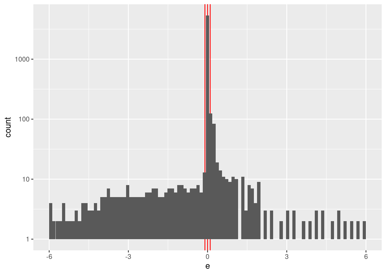
| Version | Author | Date |
|---|---|---|
| 2e83517 | Ross Gayler | 2021-09-11 |
Construct a spline specification with knots set at \({-6, -2, -0.1, 0, 0.1, 2, 6}\).
vsa_dim <- 1e4L

ss_e <- vsa_mk_scalar_encoder_spline_spec(vsa_dim = vsa_dim, knots = c(-6, -0.1, 0, 0.1, 2, 6))
In using regression to decode VSA representations I will have to create a data matrix with one row per observation (the encoding of the value \(e\)). One column will correspond to the dependent variable - the target value \(u\). The remaining columns correspond to the independent variables (predictors) - the VSA vector representation of the encoded scalar value \(e\). There will be one column for each element of the vector representation.
The number of columns will exceed the number of rows, so simple
unregularised regression will fail. I will initially attempt to use
regularised regression (elasticnet, implemented by glmnet in R).
# create the numeric scalar values to be encoded
d_subset <- d_wide %>%
  dplyr::slice_sample(n = n_samp) %>%
  dplyr::select(u, e, e_orth)

# function to to take a set of numeric scalar values,
# encode them as VSA vectors using the given spline specification,
# and package the results as a data frame for regression modelling
mk_df <- function(
  x, # numeric - vector of scalar values to be VSA encoded
  ss # data frame - spline specification for scalar encoding
) # value - data frame - one row per scalar, one column for the scalar and each VSA element
{
  tibble::tibble(x_num = x) %>% # put scalars as column of data frame
    dplyr::rowwise() %>%
    dplyr::mutate(
      x_vsa = x_num %>% vsa_encode_scalar_spline(ss) %>% # encode each scalar
        tibble(vsa_i = 1:length(.), vsa_val = .) %>% # name all the vector elements
        tidyr::pivot_wider(names_from = vsa_i, names_prefix = "vsa_", values_from = vsa_val) %>% # transpose vector to columns
        list() # package the value for a list column
    ) %>%
    dplyr::ungroup() %>%
    tidyr::unnest(x_vsa) %>%  # convert the nested df to columns
    dplyr::select(-x_num) # drop the scalar value that was encoded
}

# create training data
# contains: u, encode(e)
d_train <- dplyr::bind_cols(
  dplyr::select(d_subset, u),
  mk_df(dplyr::pull(d_subset, e), ss_e)
  )

# take a quick look at the data
d_train
# A tibble: 2,000 × 10,001
u vsa_1 vsa_2 vsa_3 vsa_4 vsa_5 vsa_6 vsa_7 vsa_8 vsa_9 vsa_10 vsa_11
<dbl> <int> <int> <int> <int> <int> <int> <int> <int> <int> <int> <int>
1 0.563 1 1 -1 -1 -1 -1 1 1 -1 1 1
2 0.527 1 1 -1 -1 -1 -1 1 1 -1 1 1
3 0.61 1 -1 1 -1 1 -1 -1 -1 -1 -1 1
4 0.575 1 -1 -1 -1 -1 -1 1 1 -1 1 1
5 0 -1 1 1 -1 1 1 1 -1 1 -1 -1
6 0.507 1 1 -1 -1 -1 -1 1 1 -1 1 1
7 0.499 1 1 -1 -1 -1 -1 1 1 -1 1 1
8 0.557 1 1 -1 -1 -1 -1 1 1 -1 1 1
9 0 -1 -1 1 -1 1 1 1 -1 1 -1 -1
10 0.534 1 1 -1 -1 -1 -1 1 1 -1 1 1
# … with 1,990 more rows, and 9,989 more variables: vsa_12 <int>, vsa_13 <int>,
# vsa_14 <int>, vsa_15 <int>, vsa_16 <int>, vsa_17 <int>, vsa_18 <int>,
# vsa_19 <int>, vsa_20 <int>, vsa_21 <int>, vsa_22 <int>, vsa_23 <int>,
# vsa_24 <int>, vsa_25 <int>, vsa_26 <int>, vsa_27 <int>, vsa_28 <int>,
# vsa_29 <int>, vsa_30 <int>, vsa_31 <int>, vsa_32 <int>, vsa_33 <int>,
# vsa_34 <int>, vsa_35 <int>, vsa_36 <int>, vsa_37 <int>, vsa_38 <int>,
# vsa_39 <int>, vsa_40 <int>, vsa_41 <int>, vsa_42 <int>, vsa_43 <int>, …# create testing data
# contains: e, encode(e)
e_test <- seq(from = -6, to = 6, by = 0.05) # grid of e values
d_test <- dplyr::bind_cols(
tibble::tibble(e = e_test),
mk_df(e_test, ss_e)
)
# take a quick look at the data
d_test# A tibble: 241 × 10,001
e vsa_1 vsa_2 vsa_3 vsa_4 vsa_5 vsa_6 vsa_7 vsa_8 vsa_9 vsa_10 vsa_11
<dbl> <int> <int> <int> <int> <int> <int> <int> <int> <int> <int> <int>
1 -6 -1 1 -1 -1 1 -1 1 1 -1 1 -1
2 -5.95 -1 1 -1 -1 1 -1 1 1 -1 1 -1
3 -5.9 -1 1 -1 -1 1 -1 1 1 -1 1 -1
4 -5.85 -1 -1 -1 -1 1 -1 1 1 -1 1 -1
5 -5.8 -1 1 -1 -1 1 -1 1 1 -1 1 -1
6 -5.75 -1 1 -1 -1 1 -1 1 1 -1 1 -1
7 -5.7 -1 1 -1 -1 1 -1 1 1 -1 1 -1
8 -5.65 -1 1 -1 -1 1 -1 1 1 -1 1 -1
9 -5.6 -1 1 -1 -1 1 -1 1 1 1 1 -1
10 -5.55 -1 1 -1 -1 1 -1 1 1 -1 -1 -1
# … with 231 more rows, and 9,989 more variables: vsa_12 <int>, vsa_13 <int>,
# vsa_14 <int>, vsa_15 <int>, vsa_16 <int>, vsa_17 <int>, vsa_18 <int>,
# vsa_19 <int>, vsa_20 <int>, vsa_21 <int>, vsa_22 <int>, vsa_23 <int>,
# vsa_24 <int>, vsa_25 <int>, vsa_26 <int>, vsa_27 <int>, vsa_28 <int>,
# vsa_29 <int>, vsa_30 <int>, vsa_31 <int>, vsa_32 <int>, vsa_33 <int>,
# vsa_34 <int>, vsa_35 <int>, vsa_36 <int>, vsa_37 <int>, vsa_38 <int>,
# vsa_39 <int>, vsa_40 <int>, vsa_41 <int>, vsa_42 <int>, vsa_43 <int>, …The data has 101 observations where each has the encoded numeric value and the 10,000 elements of the encoded VSA representation.
Fit a linear (i.e. Gaussian family) regression model, predicting the encoded numeric value from the VSA elements.
Use glmnet() because it fits regularised regressions, allowing it to
deal with the number of predictors being much greater than the number of
observations. Also, it has been engineered for efficiency with large
numbers of predictors.
glmnet() can make use of parallel processing but it’s not needed here
as this code runs sufficiently rapidly on a modest laptop computer.
cva.glmnet() in the code below runs cross-validation fits across a
grid of \(\alpha\) and \(\lambda\) values so that we can choose the best
regularisation scheme. \(\alpha = 1\) corresponds to the ridge-regression
penalty and \(\alpha = 0\) corresponds to the lasso penalty. The \(\lambda\)
parameter is the weighting of the elastic-net penalty.
I will use the cross-validation analysis to select the parameters rather than testing on a hold-out sample, because it is less programming effort and I don’t expect it to make a substantial difference to the results.
Use alpha = 0 (ridge regression)
# fit a set of models at a grid of alpha and lambda parameter values
fit_1 <- glmnetUtils::cva.glmnet(u ~ ., data = d_train, family = "gaussian", alpha = 0)
fit_1
Call:
cva.glmnet.formula(formula = u ~ ., data = d_train, family = "gaussian",
alpha = 0)
Model fitting options:
Sparse model matrix: FALSE
Use model.frame: FALSE
Alpha values: 0
Number of crossvalidation folds for lambda: 10Look at the impact of the \(\lambda\) parameter on goodness of fit for the \(\alpha = 0\) curve.
# check that we are looking at the correct curve (alpha = 0)
fit_1$alpha[1]
[1] 0# extract the alpha = 0 model
fit_1_alpha_0 <- fit_1$modlist[[1]]
# look at the lambda curve
plot(fit_1_alpha_0)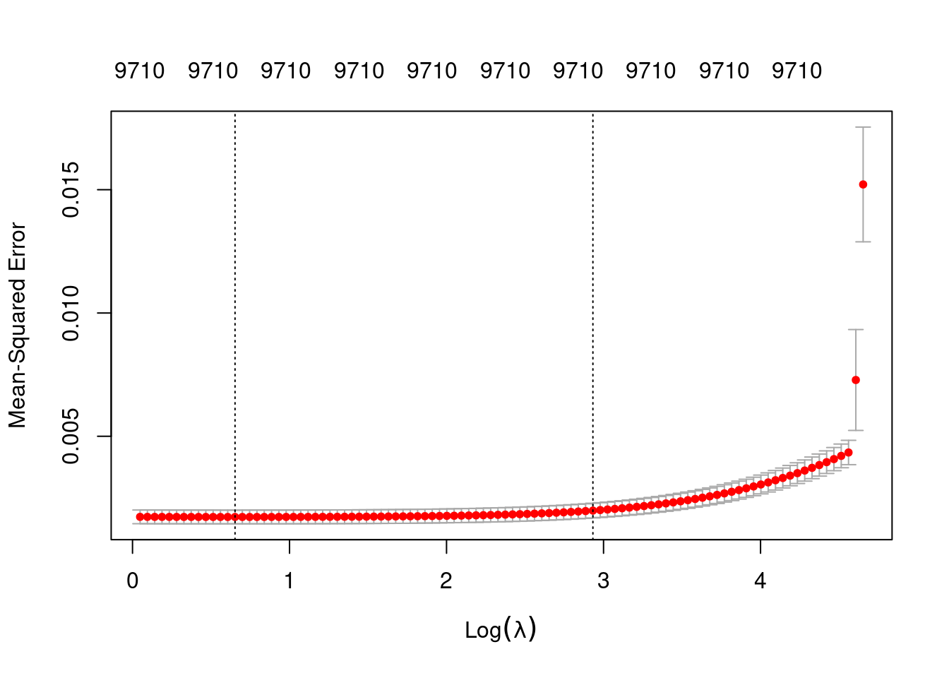
# get a summary of the alpha = 0 model
fit_1_alpha_0
Call:  glmnet::cv.glmnet(x = x, y = y, weights = ..1, offset = ..2,      nfolds = nfolds, foldid = foldid, alpha = a, family = "gaussian")

Measure: Mean-Squared Error

    Lambda Index  Measure        SE Nonzero
min  1.921    87 0.001727 0.0002776    9710
1se 18.771 38 0.001986 0.0002977 9710- The left dotted vertical line corresponds to minimum error. The right dotted vertical line corresponds to the largest value of lambda such that the error is within one standard-error of the minimum - the so-called “one-standard-error” rule.
- The numbers along the top margin show the number of nonzero coefficients in the regression models corresponding to the lambda values. All the plausible models have a number of nonzero coefficients equal to roughly half the dimensionality of the VSA vectors.
Look at the model selected by the one-standard-error rule.
First look at how good the predictions are.
# add the predicted values to the tset data frame
d_test <- d_test %>%
  dplyr::mutate(u_hat = predict(fit_1, newdata = ., alpha = 0, s = "lambda.min")) %>%
  dplyr::relocate(u_hat)

# plot of predicted u vs e
d_test %>%
  ggplot() +
  geom_vline(xintercept = c(-6, -0.1, 0, 0.1, 2, 6), colour = "skyblue3") + # knots
  geom_hline(yintercept = c(0, 1), colour = "darkgrey") + # limits of u
  geom_smooth(data = d_wide, aes(x = e, y = u), method = "gam", formula = y ~ s(x, bs = "ad", k = 150)) +
  geom_point(data = d_wide, aes(x = e, y = u), colour = "red", alpha = 0.2) +
  geom_point(aes(x = e, y = u_hat))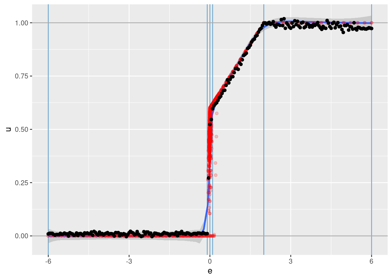
- That’s a pretty good fit.
- The slope of the fit is a little less than it should be. This is probably due to the regularisation. (The regression coefficients are shrunk towards zero.)
3 \(e_{orth}\) term
Model the marginal effect of the \(e\) term.
Check the distribution of \(e\).
summary(d_wide$e_orth) Min. 1st Qu. Median Mean 3rd Qu. Max.
-4.82950 -0.47987 0.16700 0.04648 0.70762 5.06700 d_wide %>%
ggplot2::ggplot() +
geom_vline(xintercept = c(-0.1, 0, 0.1), colour = "red") +
geom_histogram(aes(x = e_orth), bins = 100) +
scale_y_log10()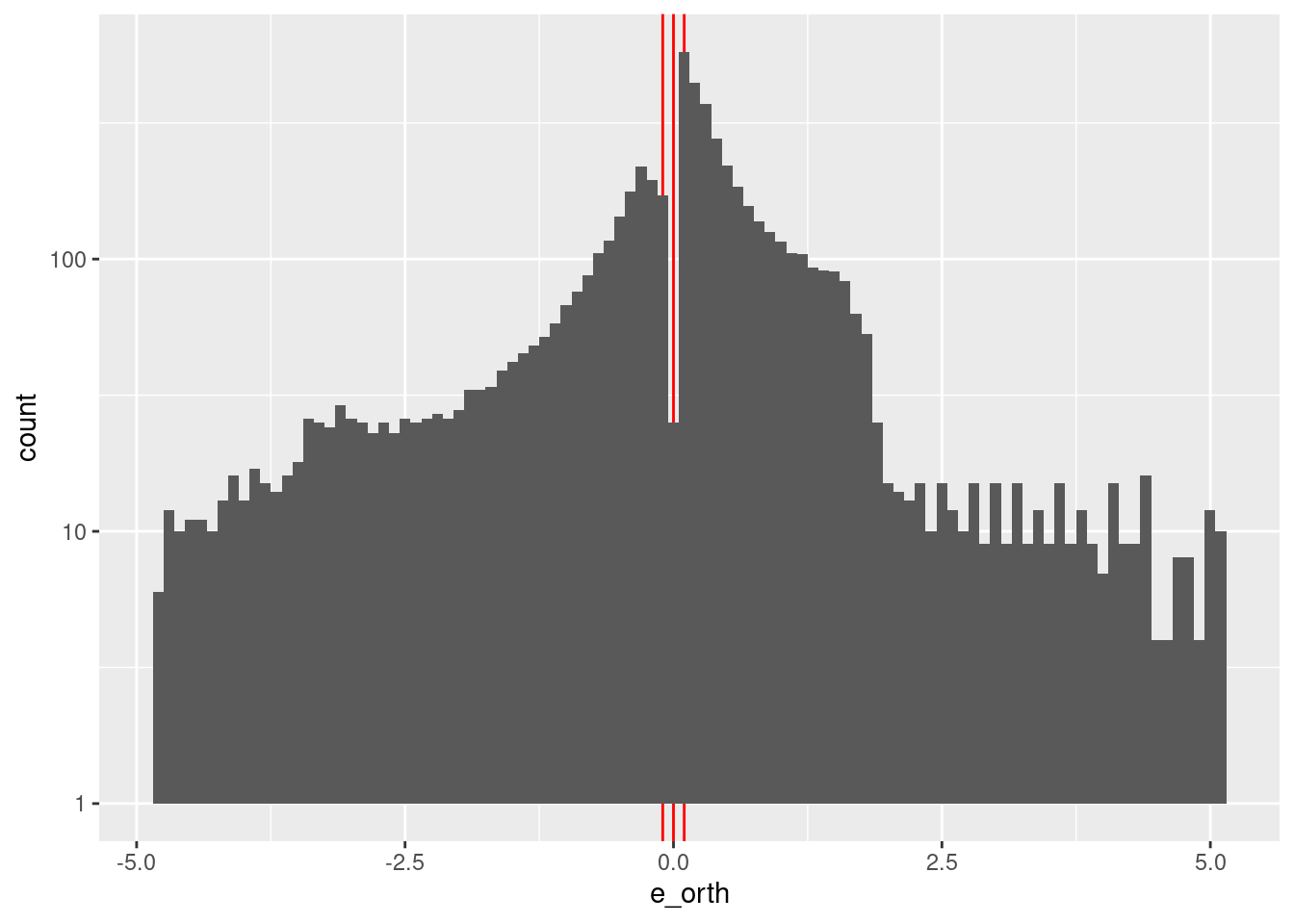
| Version | Author | Date |
|---|---|---|
| d27c378 | Ross Gayler | 2021-09-12 |
Construct a spline specification with knots set at \({-6, -2, -0.1, 0, 0.1, 2, 6}\).
ss_eo <- vsa_mk_scalar_encoder_spline_spec(vsa_dim = vsa_dim, knots = c(-5, 5))d_subset_eo <- d_subset %>%
dplyr:: filter(abs(e) < 0.1)
# create training data
# contains: u, encode(e_orth)
d_train <- dplyr::bind_cols(
dplyr::select(d_subset_eo, u),
mk_df(dplyr::pull(d_subset_eo, e_orth), ss_eo)
)
# take a quick look at the data
d_train# A tibble: 1,802 × 10,001
u vsa_1 vsa_2 vsa_3 vsa_4 vsa_5 vsa_6 vsa_7 vsa_8 vsa_9 vsa_10 vsa_11
<dbl> <int> <int> <int> <int> <int> <int> <int> <int> <int> <int> <int>
1 0.563 -1 1 1 -1 1 -1 1 1 1 1 -1
2 0.527 -1 -1 1 -1 1 -1 1 -1 -1 1 -1
3 0.61 -1 -1 1 -1 -1 -1 1 -1 1 -1 -1
4 0.575 -1 -1 1 -1 -1 -1 -1 -1 1 -1 -1
5 0.507 -1 -1 1 -1 1 -1 -1 1 1 -1 -1
6 0.499 1 -1 1 -1 -1 -1 1 -1 1 -1 -1
7 0.557 -1 -1 1 -1 -1 -1 1 -1 1 1 -1
8 0.534 -1 -1 1 -1 -1 -1 1 1 -1 1 -1
9 0.52 1 1 1 -1 1 -1 1 -1 1 1 -1
10 0.44 1 1 1 -1 -1 -1 -1 1 -1 -1 -1
# … with 1,792 more rows, and 9,989 more variables: vsa_12 <int>, vsa_13 <int>,
# vsa_14 <int>, vsa_15 <int>, vsa_16 <int>, vsa_17 <int>, vsa_18 <int>,
# vsa_19 <int>, vsa_20 <int>, vsa_21 <int>, vsa_22 <int>, vsa_23 <int>,
# vsa_24 <int>, vsa_25 <int>, vsa_26 <int>, vsa_27 <int>, vsa_28 <int>,
# vsa_29 <int>, vsa_30 <int>, vsa_31 <int>, vsa_32 <int>, vsa_33 <int>,
# vsa_34 <int>, vsa_35 <int>, vsa_36 <int>, vsa_37 <int>, vsa_38 <int>,
# vsa_39 <int>, vsa_40 <int>, vsa_41 <int>, vsa_42 <int>, vsa_43 <int>, …# create testing data
# contains: e, encode(e)
eo_test <- seq(from = -5, to = 5, by = 0.05) # grid of e_orth values
d_test <- dplyr::bind_cols(
tibble::tibble(e_orth = eo_test),
mk_df(eo_test, ss_eo)
)
# take a quick look at the data
d_test# A tibble: 201 × 10,001
e_orth vsa_1 vsa_2 vsa_3 vsa_4 vsa_5 vsa_6 vsa_7 vsa_8 vsa_9 vsa_10 vsa_11
<dbl> <int> <int> <int> <int> <int> <int> <int> <int> <int> <int> <int>
1 -5 -1 -1 1 -1 -1 -1 1 -1 1 1 -1
2 -4.95 -1 -1 1 -1 -1 -1 1 -1 1 1 -1
3 -4.9 -1 -1 1 -1 -1 -1 1 -1 1 1 -1
4 -4.85 -1 -1 1 -1 -1 -1 1 -1 1 1 -1
5 -4.8 -1 -1 1 -1 -1 -1 1 -1 -1 1 -1
6 -4.75 -1 -1 1 -1 -1 -1 1 -1 1 1 -1
7 -4.7 -1 -1 1 -1 -1 -1 1 -1 1 1 -1
8 -4.65 -1 1 1 -1 -1 -1 1 -1 1 1 -1
9 -4.6 -1 -1 1 -1 -1 -1 1 -1 1 1 -1
10 -4.55 -1 -1 1 -1 -1 -1 1 -1 1 1 -1
# … with 191 more rows, and 9,989 more variables: vsa_12 <int>, vsa_13 <int>,
# vsa_14 <int>, vsa_15 <int>, vsa_16 <int>, vsa_17 <int>, vsa_18 <int>,
# vsa_19 <int>, vsa_20 <int>, vsa_21 <int>, vsa_22 <int>, vsa_23 <int>,
# vsa_24 <int>, vsa_25 <int>, vsa_26 <int>, vsa_27 <int>, vsa_28 <int>,
# vsa_29 <int>, vsa_30 <int>, vsa_31 <int>, vsa_32 <int>, vsa_33 <int>,
# vsa_34 <int>, vsa_35 <int>, vsa_36 <int>, vsa_37 <int>, vsa_38 <int>,
# vsa_39 <int>, vsa_40 <int>, vsa_41 <int>, vsa_42 <int>, vsa_43 <int>, …# fit a set of models at a grid of alpha and lambda parameter values
fit_2 <- glmnetUtils::cva.glmnet(u ~ ., data = d_train, family = "gaussian", alpha = 0)
fit_2Call:
cva.glmnet.formula(formula = u ~ ., data = d_train, family = "gaussian",
alpha = 0)
Model fitting options:
Sparse model matrix: FALSE
Use model.frame: FALSE
Alpha values: 0
Number of crossvalidation folds for lambda: 10Look at the impact of the \(\lambda\) parameter on goodness of fit for the \(\alpha = 0\) curve.
# check that we are looking at the correct curve (alpha = 0)
fit_2$alpha[1]
[1] 0# extract the alpha = 0 model
fit_2_alpha_0 <- fit_2$modlist[[1]]
# look at the lambda curve
plot(fit_2_alpha_0)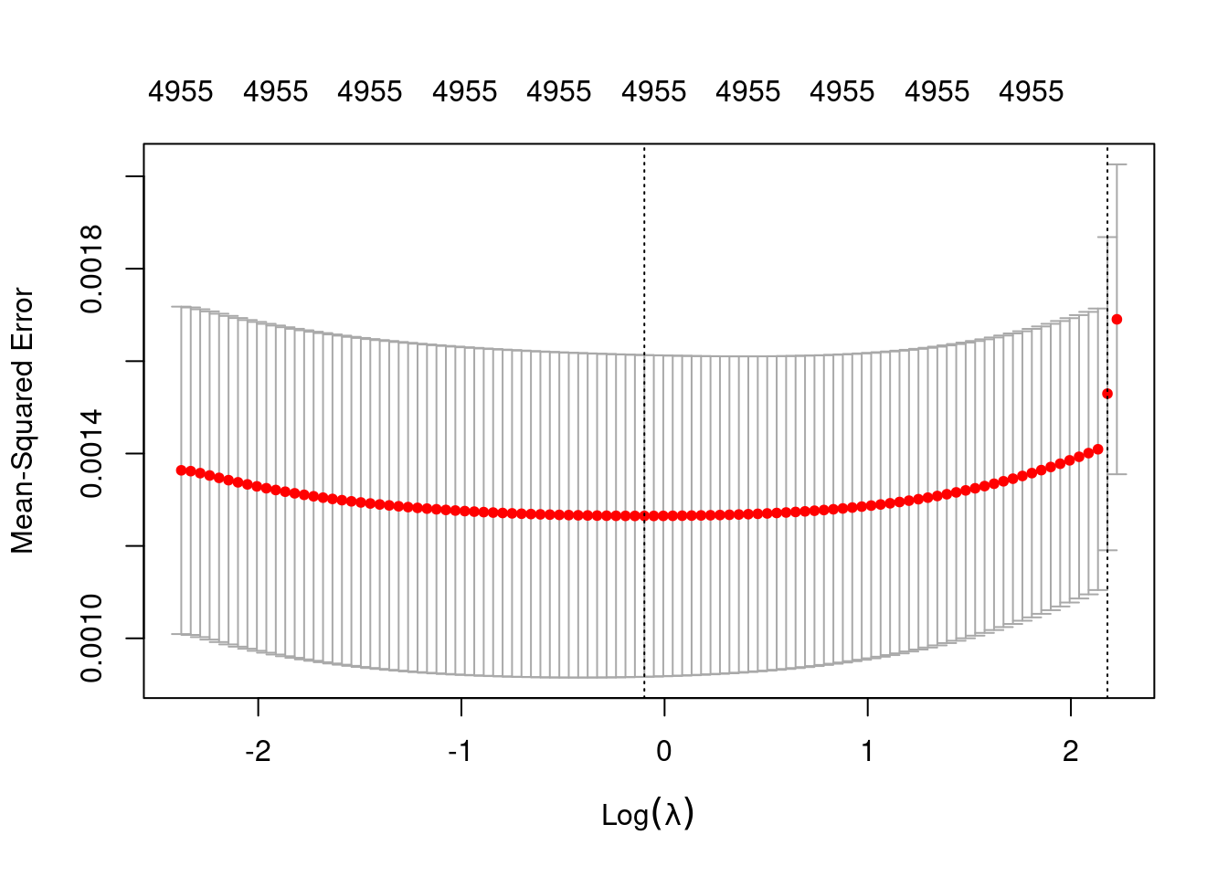
# get a summary of the alpha = 0 model
fit_2_alpha_0
Call:  glmnet::cv.glmnet(x = x, y = y, weights = ..1, offset = ..2,      nfolds = nfolds, foldid = foldid, alpha = a, family = "gaussian")

Measure: Mean-Squared Error

    Lambda Index  Measure        SE Nonzero
min  0.905    51 0.001265 0.0003482    4955
1se 8.845 2 0.001530 0.0003389 4955- The left dotted vertical line corresponds to minimum error. The right dotted vertical line corresponds to the largest value of lambda such that the error is within one standard-error of the minimum - the so-called “one-standard-error” rule.
- The numbers along the top margin show the number of nonzero coefficients in the regression models corresponding to the lambda values. All the plausible models have a number of nonzero coefficients equal to roughly half the dimensionality of the VSA vectors.
Look at the model selected by the one-standard-error rule.
First look at how good the predictions are.
# add the predicted values to the tset data frame
d_test <- d_test %>%
  dplyr::mutate(u_hat = predict(fit_2, newdata = ., alpha = 0, s = "lambda.min")) %>%
  dplyr::relocate(u_hat)

# plot of predicted u vs e
d_test %>%
  ggplot() +
  geom_vline(xintercept = c(-5, 5), colour = "skyblue3") + # knots
  geom_hline(yintercept = c(0, 1), colour = "darkgrey") + # limits of u
  # geom_smooth(data = dplyr::filter(d_wide, abs(e) < 0.1), aes(x = e_orth, y = u), method = "gam", formula = y ~ s(x, bs = "ad")) +
  geom_point(data = dplyr::filter(d_wide, abs(e) < 0.1), aes(x = e_orth, y = u), colour = "red", alpha = 0.2) +
  geom_point(aes(x = e_orth, y = u_hat))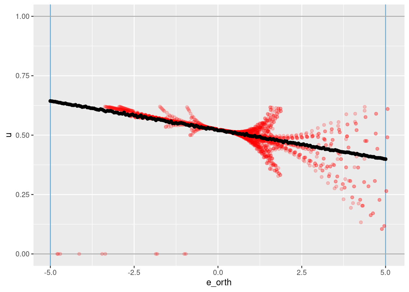
4 Joint \(e\) and \(e_{orth}\) term
Model the marginal effect of the \(e\) term.
# function to to take a set of numeric scalar values,
# encode them as VSA vectors using the given spline specification,
# and package the results as a data frame for regression modelling
mk_df_j <- function(
  x_e, # numeric - vector of scalar values to be VSA encoded
  x_eo,
  ss_e,
  ss_eo# data frame - spline specification for scalar encoding
) # value - data frame - one row per scalar, one column for the scalar and each VSA element
{
  tibble::tibble(x_e = x_e, x_eo = x_eo) %>% # put scalars as column of data frame
    dplyr::rowwise() %>%
    dplyr::mutate(
      x_vsa = vsa_multiply(
        vsa_encode_scalar_spline(x_e, ss_e),
        vsa_encode_scalar_spline(x_eo, ss_eo)
      ) %>%
        tibble(vsa_i = 1:length(.), vsa_val = .) %>% # name all the vector elements
        tidyr::pivot_wider(names_from = vsa_i, names_prefix = "vsa_", values_from = vsa_val) %>% # transpose vector to columns
        list() # package the value for a list column
    ) %>%
    dplyr::ungroup() %>%
    tidyr::unnest(x_vsa) %>%  # convert the nested df to columns
    dplyr::select(-x_e, -x_eo) # drop the scalar value that was encoded
}

# create training data
# contains: u, encode(e)
d_train <- dplyr::bind_cols(
  dplyr::select(d_subset, u),
  mk_df_j(dplyr::pull(d_subset, e), dplyr::pull(d_subset, e_orth), ss_e, ss_eo)
)

# take a quick look at the data
d_train
# A tibble: 2,000 × 10,001
u vsa_1 vsa_2 vsa_3 vsa_4 vsa_5 vsa_6 vsa_7 vsa_8 vsa_9 vsa_10 vsa_11
<dbl> <int> <int> <int> <int> <int> <int> <int> <int> <int> <int> <int>
1 0.563 -1 -1 -1 1 1 1 -1 1 -1 1 -1
2 0.527 1 1 -1 1 -1 1 1 -1 -1 1 -1
3 0.61 -1 -1 -1 -1 -1 1 -1 -1 -1 1 -1
4 0.575 1 -1 -1 1 1 1 -1 1 -1 1 -1
5 0 -1 -1 1 1 -1 1 1 1 1 -1 1
6 0.507 1 1 -1 1 -1 1 -1 1 -1 -1 -1
7 0.499 -1 1 -1 1 -1 1 1 1 1 -1 -1
8 0.557 -1 -1 -1 1 1 1 1 1 1 1 -1
9 0 -1 1 1 1 -1 -1 1 1 -1 1 1
10 0.534 -1 1 -1 1 -1 1 1 -1 -1 1 -1
# … with 1,990 more rows, and 9,989 more variables: vsa_12 <int>, vsa_13 <int>,
# vsa_14 <int>, vsa_15 <int>, vsa_16 <int>, vsa_17 <int>, vsa_18 <int>,
# vsa_19 <int>, vsa_20 <int>, vsa_21 <int>, vsa_22 <int>, vsa_23 <int>,
# vsa_24 <int>, vsa_25 <int>, vsa_26 <int>, vsa_27 <int>, vsa_28 <int>,
# vsa_29 <int>, vsa_30 <int>, vsa_31 <int>, vsa_32 <int>, vsa_33 <int>,
# vsa_34 <int>, vsa_35 <int>, vsa_36 <int>, vsa_37 <int>, vsa_38 <int>,
# vsa_39 <int>, vsa_40 <int>, vsa_41 <int>, vsa_42 <int>, vsa_43 <int>, …# create testing data
# contains: e, encode(e)
e_test <- c(seq(from = -6, to = -1, by = 1), seq(from = -0.2, to = 0.2, by = 0.05), seq(from = 1, to = 6, by = 1)) # grid of e values
eo_test <- seq(from = -5, to = 5, by = 1) # grid of e values
d_grid <- tidyr::expand_grid(e = e_test, e_orth = eo_test)
d_test <- dplyr::bind_cols(
d_grid,
mk_df_j(dplyr::pull(d_grid, e), dplyr::pull(d_grid, e_orth), ss_e, ss_eo)
)
# take a quick look at the data
d_test# A tibble: 231 × 10,002
e e_orth vsa_1 vsa_2 vsa_3 vsa_4 vsa_5 vsa_6 vsa_7 vsa_8 vsa_9 vsa_10
<dbl> <dbl> <int> <int> <int> <int> <int> <int> <int> <int> <int> <int>
1 -6 -5 1 -1 -1 1 -1 1 1 -1 -1 1
2 -6 -4 1 -1 -1 1 -1 1 1 1 -1 1
3 -6 -3 -1 -1 -1 1 -1 1 1 1 -1 1
4 -6 -2 1 -1 -1 1 -1 1 1 1 -1 1
5 -6 -1 -1 1 -1 1 -1 1 1 1 -1 1
6 -6 0 1 1 -1 1 -1 1 1 -1 -1 1
7 -6 1 -1 -1 -1 1 1 1 -1 -1 -1 -1
8 -6 2 -1 1 -1 1 -1 1 -1 1 -1 -1
9 -6 3 -1 -1 -1 1 1 1 -1 1 1 -1
10 -6 4 -1 1 -1 1 1 1 -1 1 -1 -1
# … with 221 more rows, and 9,990 more variables: vsa_11 <int>, vsa_12 <int>,
# vsa_13 <int>, vsa_14 <int>, vsa_15 <int>, vsa_16 <int>, vsa_17 <int>,
# vsa_18 <int>, vsa_19 <int>, vsa_20 <int>, vsa_21 <int>, vsa_22 <int>,
# vsa_23 <int>, vsa_24 <int>, vsa_25 <int>, vsa_26 <int>, vsa_27 <int>,
# vsa_28 <int>, vsa_29 <int>, vsa_30 <int>, vsa_31 <int>, vsa_32 <int>,
# vsa_33 <int>, vsa_34 <int>, vsa_35 <int>, vsa_36 <int>, vsa_37 <int>,
# vsa_38 <int>, vsa_39 <int>, vsa_40 <int>, vsa_41 <int>, vsa_42 <int>, …# fit a set of models at a grid of alpha and lambda parameter values
fit_3 <- glmnetUtils::cva.glmnet(u ~ ., data = d_train, family = "gaussian", alpha = 0)
fit_3Call:
cva.glmnet.formula(formula = u ~ ., data = d_train, family = "gaussian",
alpha = 0)
Model fitting options:
Sparse model matrix: FALSE
Use model.frame: FALSE
Alpha values: 0
Number of crossvalidation folds for lambda: 10Look at the impact of the \(\lambda\) parameter on goodness of fit for the \(\alpha = 0\) curve.
# check that we are looking at the correct curve (alpha = 0)
fit_3$alpha[1]
[1] 0# extract the alpha = 0 model
fit_3_alpha_0 <- fit_3$modlist[[1]]
# look at the lambda curve
plot(fit_3_alpha_0)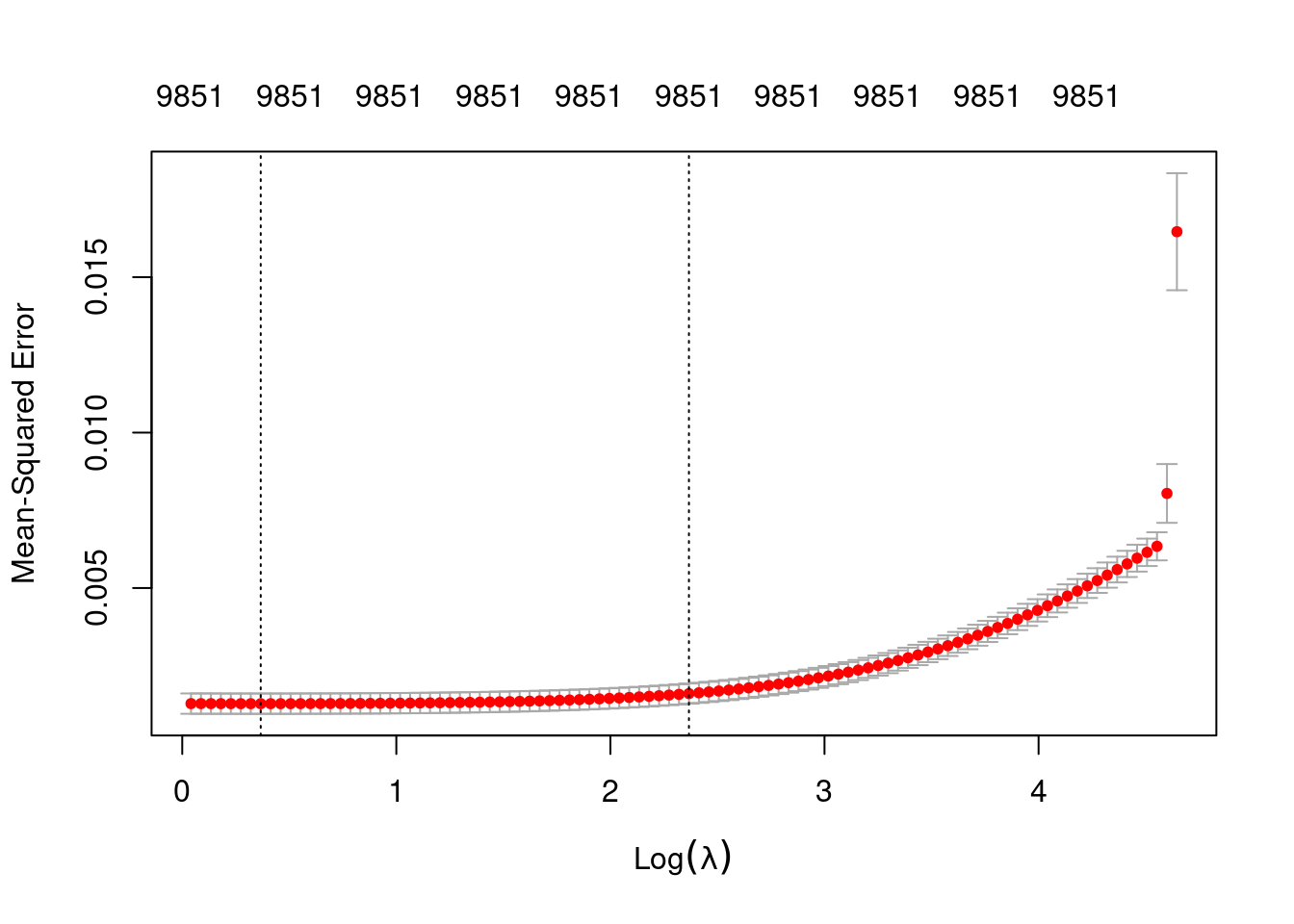
| Version | Author | Date |
|---|---|---|
| bf544c6 | Ross Gayler | 2021-09-12 |
# get a summary of the alpha = 0 model
fit_3_alpha_0
Call:  glmnet::cv.glmnet(x = x, y = y, weights = ..1, offset = ..2,      nfolds = nfolds, foldid = foldid, alpha = a, family = "gaussian")

Measure: Mean-Squared Error

    Lambda Index  Measure        SE Nonzero
min  1.443    93 0.001279 0.0003275    9851
1se 10.664 50 0.001604 0.0003244 9851- The left dotted vertical line corresponds to minimum error. The right dotted vertical line corresponds to the largest value of lambda such that the error is within one standard-error of the minimum - the so-called “one-standard-error” rule.
- The numbers along the top margin show the number of nonzero coefficients in the regression models corresponding to the lambda values. All the plausible models have a number of nonzero coefficients equal to roughly half the dimensionality of the VSA vectors.
Look at the model selected by the one-standard-error rule.
First look at how good the predictions are.
# add the predicted values to the tset data frame
d_test <- d_test %>%
  dplyr::mutate(u_hat = predict(fit_3, newdata = ., alpha = 0, s = "lambda.min")) %>%
  dplyr::relocate(u_hat)

# plot of predicted u vs e
d_test %>%
  ggplot() +
  geom_point(aes(x = e, y = e_orth, size = u_hat, colour = u_hat)) +
  scale_color_viridis_c()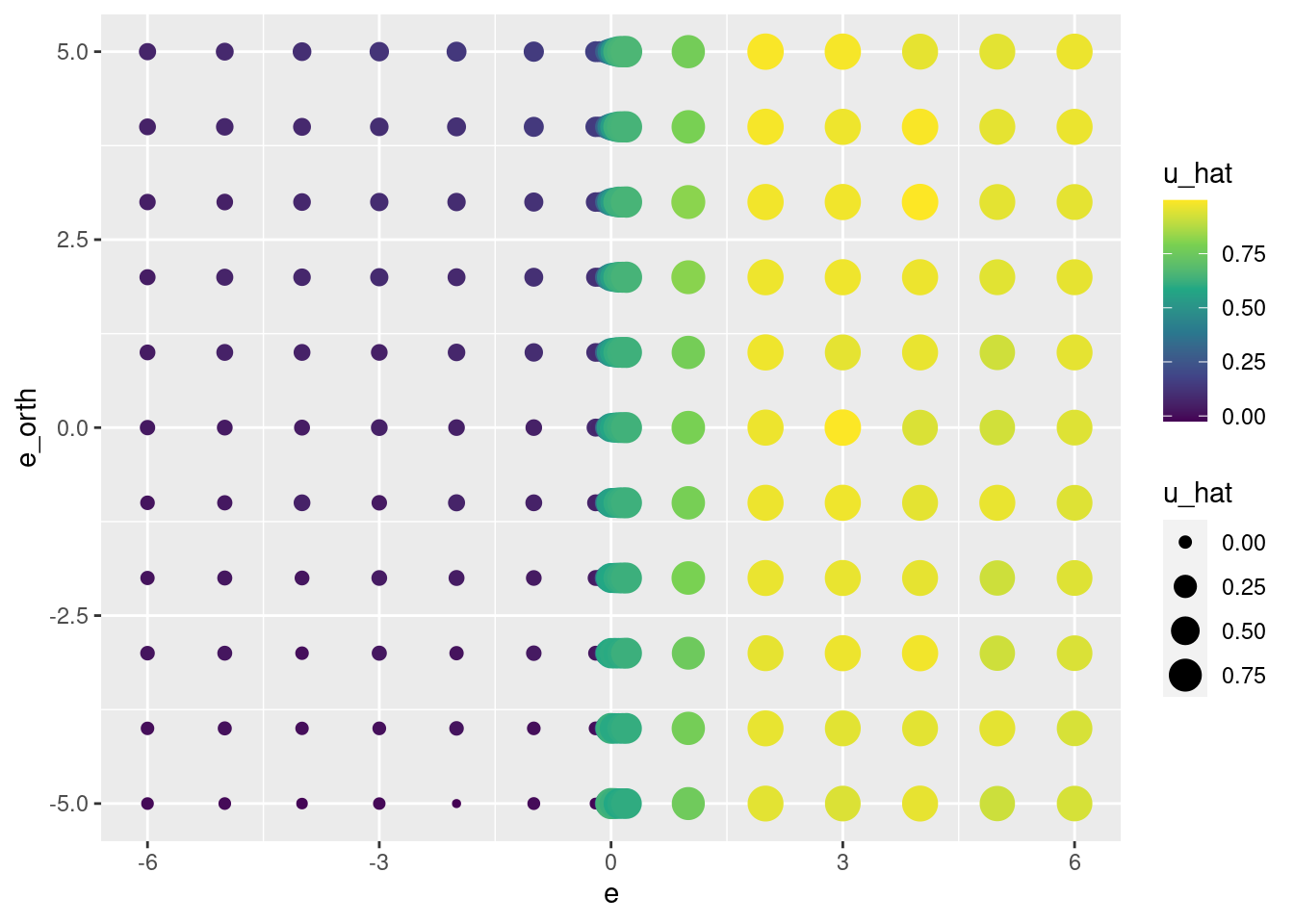
| Version | Author | Date |
|---|---|---|
| bf544c6 | Ross Gayler | 2021-09-12 |
lattice::wireframe(u_hat ~ e * e_orth, data = d_test, drape = TRUE)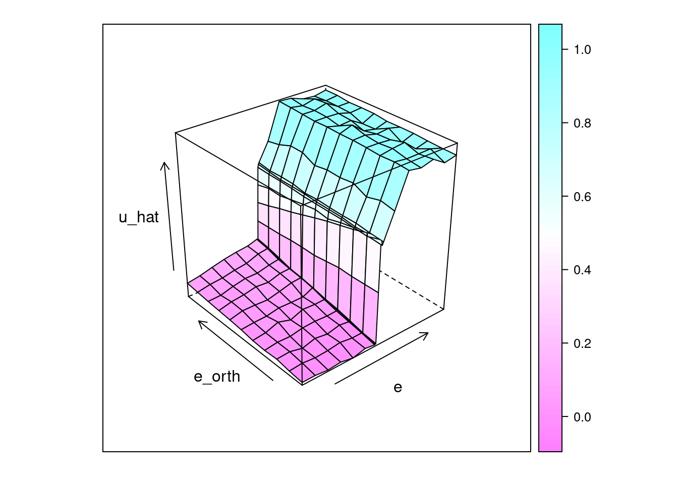
| Version | Author | Date |
|---|---|---|
| bf544c6 | Ross Gayler | 2021-09-12 |
d_test %>%
  ggplot() +
  geom_point(aes(x = e_orth, y = u_hat)) +
  facet_wrap(facets = vars(e))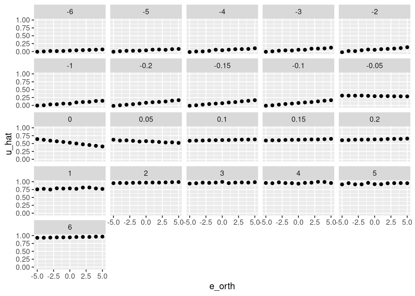
| Version | Author | Date |
|---|---|---|
| bf544c6 | Ross Gayler | 2021-09-12 |
5 Joint \(k_{tgt}\), \(z\), and \(dz\) term
Model the marginal effect of the \(e\) term.
Check the distribution of input variables.
summary(d_wide$k_tgt) Min. 1st Qu. Median Mean 3rd Qu. Max.
1.000 2.000 4.000 4.001 5.000 8.000 d_wide %>%
ggplot2::ggplot() +
geom_histogram(aes(x = k_tgt), bins = 100)
summary(d_wide$z) Min. 1st Qu. Median Mean 3rd Qu. Max.
1.079 2.549 3.807 3.979 5.086 7.926 d_wide %>%
ggplot2::ggplot() +
geom_histogram(aes(x = z), bins = 100) +
scale_y_log10()
summary(d_wide$dz) Min. 1st Qu. Median Mean 3rd Qu. Max.
-4.9950 -0.4522 0.1640 0.0708 0.6793 5.0730 d_wide %>%
ggplot2::ggplot() +
geom_histogram(aes(x = dz), bins = 100) +
scale_y_log10()
Construct a spline specification with knots set at \({-6, -2, -0.1, 0, 0.1, 2, 6}\).
ss_tgt <- vsa_mk_scalar_encoder_spline_spec(vsa_dim = vsa_dim, knots = seq(from = 1, to = 8, by = 0.5))
ss_z <- vsa_mk_scalar_encoder_spline_spec(vsa_dim = vsa_dim, knots = seq(from = 1, to = 8, by = 0.5))
ss_dz <- vsa_mk_scalar_encoder_spline_spec(vsa_dim = vsa_dim, knots = seq(from = -5, to = 5, by = 0.5))
d_subset <- d_wide %>%
dplyr::slice_sample(n = n_samp) %>%
dplyr::select(u, e, e_orth, k_tgt, z, dz)
# function to to take a set of numeric scalar values,
# encode them as VSA vectors using the given spline specification,
# and package the results as a data frame for regression modelling
mk_df_j3 <- function(
x_tgt, # numeric - vector of scalar values to be VSA encoded
x_z,
x_dz,
ss_tgt,
ss_z,
ss_dz # data frame - spline specification for scalar encoding
) # value - data frame - one row per scalar, one column for the scalar and each VSA element
{
tibble::tibble(x_tgt = x_tgt, x_z = x_z, x_dz = x_dz) %>% # put scalars as column of data frame
dplyr::rowwise() %>%
dplyr::mutate(
x_vsa = vsa_multiply(
vsa_encode_scalar_spline(x_tgt, ss_tgt),
vsa_encode_scalar_spline(x_z, ss_z),
vsa_encode_scalar_spline(x_dz, ss_dz)
) %>%
tibble(vsa_i = 1:length(.), vsa_val = .) %>% # name all the vector elements
tidyr::pivot_wider(names_from = vsa_i, names_prefix = "vsa_", values_from = vsa_val) %>% # transpose vector to columns
list() # package the value for a list column
) %>%
dplyr::ungroup() %>%
tidyr::unnest(x_vsa) %>% # convert the nested df to columns
dplyr::select(-x_tgt, -x_z, -x_dz) # drop the scalar value that was encoded
}
# create training data
# contains: u, encode(e)
d_train <- dplyr::bind_cols(
dplyr::select(d_subset, u),
mk_df_j3(dplyr::pull(d_subset, k_tgt), dplyr::pull(d_subset, z), dplyr::pull(d_subset, dz), ss_tgt, ss_z, ss_dz)
)
# take a quick look at the data
d_train# A tibble: 2,000 × 10,001
u vsa_1 vsa_2 vsa_3 vsa_4 vsa_5 vsa_6 vsa_7 vsa_8 vsa_9 vsa_10 vsa_11
<dbl> <int> <int> <int> <int> <int> <int> <int> <int> <int> <int> <int>
1 0.501 -1 1 1 -1 -1 1 -1 -1 -1 1 -1
2 0.573 -1 -1 -1 -1 -1 1 -1 -1 -1 1 -1
3 0.517 -1 -1 -1 -1 1 1 -1 -1 1 1 -1
4 0.543 1 -1 1 -1 -1 1 -1 -1 -1 1 1
5 0.515 -1 1 -1 -1 1 -1 1 1 1 -1 -1
6 0.546 -1 -1 1 -1 1 -1 1 1 1 -1 -1
7 0.577 -1 1 -1 -1 -1 -1 1 1 -1 1 -1
8 0.545 -1 -1 -1 -1 1 -1 -1 1 -1 1 -1
9 0.515 -1 1 1 -1 -1 1 -1 1 -1 1 -1
10 0.535 -1 -1 1 -1 -1 1 1 -1 1 1 -1
# … with 1,990 more rows, and 9,989 more variables: vsa_12 <int>, vsa_13 <int>,
# vsa_14 <int>, vsa_15 <int>, vsa_16 <int>, vsa_17 <int>, vsa_18 <int>,
# vsa_19 <int>, vsa_20 <int>, vsa_21 <int>, vsa_22 <int>, vsa_23 <int>,
# vsa_24 <int>, vsa_25 <int>, vsa_26 <int>, vsa_27 <int>, vsa_28 <int>,
# vsa_29 <int>, vsa_30 <int>, vsa_31 <int>, vsa_32 <int>, vsa_33 <int>,
# vsa_34 <int>, vsa_35 <int>, vsa_36 <int>, vsa_37 <int>, vsa_38 <int>,
# vsa_39 <int>, vsa_40 <int>, vsa_41 <int>, vsa_42 <int>, vsa_43 <int>, …# create testing data
# contains: e, encode(e)
tgt_test <- 1:8 # grid of e values
z_test <- seq(from = 1, to = 8, by = 0.5) # grid of e values
dz_test <- seq(from = -5, to = 5, by = 0.5)
d_grid <- tidyr::expand_grid(k_tgt = tgt_test, z = z_test, dz = dz_test) %>%
dplyr::mutate(
i1 = k_tgt - z,
e = i1 - dz,
e_orth = (i1 + dz)/2
)
d_test <- dplyr::bind_cols(
d_grid,
mk_df_j3(dplyr::pull(d_grid, k_tgt), dplyr::pull(d_grid, z), dplyr::pull(d_grid, dz), ss_tgt, ss_z, ss_dz)
)
# take a quick look at the data
d_test# A tibble: 2,520 × 10,006
k_tgt z dz i1 e e_orth vsa_1 vsa_2 vsa_3 vsa_4 vsa_5 vsa_6
<int> <dbl> <dbl> <dbl> <dbl> <dbl> <int> <int> <int> <int> <int> <int>
1 1 1 -5 0 5 -2.5 -1 -1 1 -1 1 1
2 1 1 -4.5 0 4.5 -2.25 1 1 -1 -1 -1 -1
3 1 1 -4 0 4 -2 1 -1 -1 -1 -1 1
4 1 1 -3.5 0 3.5 -1.75 -1 1 1 1 1 1
5 1 1 -3 0 3 -1.5 1 1 1 1 1 -1
6 1 1 -2.5 0 2.5 -1.25 -1 1 1 -1 1 1
7 1 1 -2 0 2 -1 -1 1 -1 1 -1 1
8 1 1 -1.5 0 1.5 -0.75 1 1 -1 -1 1 1
9 1 1 -1 0 1 -0.5 1 1 1 -1 1 1
10 1 1 -0.5 0 0.5 -0.25 1 -1 1 -1 1 1
# … with 2,510 more rows, and 9,994 more variables: vsa_7 <int>, vsa_8 <int>,
# vsa_9 <int>, vsa_10 <int>, vsa_11 <int>, vsa_12 <int>, vsa_13 <int>,
# vsa_14 <int>, vsa_15 <int>, vsa_16 <int>, vsa_17 <int>, vsa_18 <int>,
# vsa_19 <int>, vsa_20 <int>, vsa_21 <int>, vsa_22 <int>, vsa_23 <int>,
# vsa_24 <int>, vsa_25 <int>, vsa_26 <int>, vsa_27 <int>, vsa_28 <int>,
# vsa_29 <int>, vsa_30 <int>, vsa_31 <int>, vsa_32 <int>, vsa_33 <int>,
# vsa_34 <int>, vsa_35 <int>, vsa_36 <int>, vsa_37 <int>, vsa_38 <int>, …# fit a set of models at a grid of alpha and lambda parameter values
fit_4 <- glmnetUtils::cva.glmnet(u ~ ., data = d_train, family = "gaussian", alpha = 0)
fit_4Call:
cva.glmnet.formula(formula = u ~ ., data = d_train, family = "gaussian",
alpha = 0)
Model fitting options:
Sparse model matrix: FALSE
Use model.frame: FALSE
Alpha values: 0
Number of crossvalidation folds for lambda: 10Look at the impact of the \(\lambda\) parameter on goodness of fit for the \(\alpha = 0\) curve.
# check that we are looking at the correct curve (alpha = 0)
fit_4$alpha[1]
[1] 0# extract the alpha = 0 model
fit_4_alpha_0 <- fit_4$modlist[[1]]
# look at the lambda curve
plot(fit_4_alpha_0)
# get a summary of the alpha = 0 model
fit_4_alpha_0
Call:  glmnet::cv.glmnet(x = x, y = y, weights = ..1, offset = ..2,      nfolds = nfolds, foldid = foldid, alpha = a, family = "gaussian")

Measure: Mean-Squared Error

    Lambda Index  Measure        SE Nonzero
min  0.213   100 0.006755 0.0004437   10000
1se 0.390 87 0.007174 0.0005087 10000- The left dotted vertical line corresponds to minimum error. The right dotted vertical line corresponds to the largest value of lambda such that the error is within one standard-error of the minimum - the so-called “one-standard-error” rule.
- The numbers along the top margin show the number of nonzero coefficients in the regression models corresponding to the lambda values. All the plausible models have a number of nonzero coefficients equal to roughly half the dimensionality of the VSA vectors.
Look at the model selected by the one-standard-error rule.
First look at how good the predictions are.
# add the predicted values to the tset data frame
d_test <- d_test %>%
  dplyr::mutate(u_hat = predict(fit_4, newdata = ., alpha = 0, s = "lambda.min")) %>%
  dplyr::relocate(u_hat)

summary(d_test$u_hat)
lambda.min
Min. :0.0268
1st Qu.:0.4464
Median :0.4738
Mean :0.4716
3rd Qu.:0.5002
Max. :0.8948 d_test %>%
ggplot2::ggplot() +
geom_histogram(aes(x = u_hat), bins = 100) +
scale_y_log10()Warning: Transformation introduced infinite values in continuous y-axisWarning: Removed 17 rows containing missing values (geom_bar).
# plot of predicted u vs e
d_test %>%
  ggplot() +
  geom_point(aes(x = e, y = e_orth, size = u_hat, colour = u_hat)) +
  scale_color_viridis_c() +
  facet_wrap(facets = vars(k_tgt))
d_test %>%
  ggplot() +
  geom_point(aes(x = e, y = u_hat)) +
  geom_smooth(aes(x = e, y = u_hat)) +
  facet_wrap(facets = vars(k_tgt))
`geom_smooth()` using method = 'loess' and formula 'y ~ x'
d_test %>%
  dplyr::filter(abs(e) < 0.1) %>%
  ggplot() +
  geom_point(aes(x = e_orth, y = u_hat)) +
  geom_smooth(aes(x = e_orth, y = u_hat), method = "lm") +
  facet_wrap(facets = vars(k_tgt))
`geom_smooth()` using formula 'y ~ x'
sessionInfo()R version 4.1.1 (2021-08-10)
Platform: x86_64-pc-linux-gnu (64-bit)
Running under: Ubuntu 21.04
Matrix products: default
BLAS: /usr/lib/x86_64-linux-gnu/blas/libblas.so.3.9.0
LAPACK: /usr/lib/x86_64-linux-gnu/lapack/liblapack.so.3.9.0
locale:
[1] LC_CTYPE=en_AU.UTF-8 LC_NUMERIC=C
[3] LC_TIME=en_AU.UTF-8 LC_COLLATE=en_AU.UTF-8
[5] LC_MONETARY=en_AU.UTF-8 LC_MESSAGES=en_AU.UTF-8
[7] LC_PAPER=en_AU.UTF-8 LC_NAME=C
[9] LC_ADDRESS=C LC_TELEPHONE=C
[11] LC_MEASUREMENT=en_AU.UTF-8 LC_IDENTIFICATION=C
attached base packages:
[1] stats graphics grDevices datasets utils methods base
other attached packages:
[1] purrr_0.3.4 DiagrammeR_1.0.6.1 lattice_0.20-44 glmnetUtils_1.1.8
[5] glmnet_4.1-2 Matrix_1.3-4 tidyr_1.1.3 tibble_3.1.4
[9] ggplot2_3.3.5 stringr_1.4.0 dplyr_1.0.7 vroom_1.5.4
[13] here_1.0.1 fs_1.5.0
loaded via a namespace (and not attached):
[1] Rcpp_1.0.7 visNetwork_2.0.9 rprojroot_2.0.2 digest_0.6.27
[5] foreach_1.5.1 utf8_1.2.2 R6_2.5.1 evaluate_0.14
[9] highr_0.9 pillar_1.6.2 rlang_0.4.11 rstudioapi_0.13
[13] whisker_0.4 rmarkdown_2.10 labeling_0.4.2 splines_4.1.1
[17] htmlwidgets_1.5.4 bit_4.0.4 munsell_0.5.0 compiler_4.1.1
[21] httpuv_1.6.3 xfun_0.25 pkgconfig_2.0.3 shape_1.4.6
[25] mgcv_1.8-36 htmltools_0.5.2 tidyselect_1.1.1 bookdown_0.24
[29] workflowr_1.6.2 codetools_0.2-18 viridisLite_0.4.0 fansi_0.5.0
[33] crayon_1.4.1 tzdb_0.1.2 withr_2.4.2 later_1.3.0
[37] grid_4.1.1 nlme_3.1-153 jsonlite_1.7.2 gtable_0.3.0
[41] lifecycle_1.0.0 git2r_0.28.0 magrittr_2.0.1 scales_1.1.1
[45] cli_3.0.1 stringi_1.7.4 farver_2.1.0 renv_0.14.0
[49] promises_1.2.0.1 ellipsis_0.3.2 generics_0.1.0 vctrs_0.3.8
[53] RColorBrewer_1.1-2 iterators_1.0.13 tools_4.1.1 bit64_4.0.5
[57] glue_1.4.2 parallel_4.1.1 fastmap_1.1.0 survival_3.2-13
[61] yaml_2.2.1 colorspace_2.0-2 knitr_1.34