Last updated: 2021-08-17

Checks: 7 0

Knit directory: VSA_altitude_hold/

This reproducible R Markdown analysis was created with workflowr (version 1.6.2). The Checks tab describes the reproducibility checks that were applied when the results were created. The Past versions tab lists the development history.

R Markdown file: up-to-date

Great! Since the R Markdown file has been committed to the Git repository, you know the exact version of the code that produced these results.

Environment: empty

Great job! The global environment was empty. Objects defined in the global environment can affect the analysis in your R Markdown file in unknown ways. For reproduciblity it’s best to always run the code in an empty environment.

Seed: set.seed(20210617)

The command set.seed(20210617) was run prior to running the code in the R Markdown file. Setting a seed ensures that any results that rely on randomness, e.g. subsampling or permutations, are reproducible.

Session information: recorded

Great job! Recording the operating system, R version, and package versions is critical for reproducibility.

Cache: none

Nice! There were no cached chunks for this analysis, so you can be confident that you successfully produced the results during this run.

File paths: relative

Great job! Using relative paths to the files within your workflowr project makes it easier to run your code on other machines.

Repository version: e19cb7e

Great! You are using Git for version control. Tracking code development and connecting the code version to the results is critical for reproducibility.

The results in this page were generated with repository version e19cb7e. See the Past versions tab to see a history of the changes made to the R Markdown and HTML files.

Note that you need to be careful to ensure that all relevant files for the analysis have been committed to Git prior to generating the results (you can use wflow_publish or wflow_git_commit). workflowr only checks the R Markdown file, but you know if there are other scripts or data files that it depends on. Below is the status of the Git repository when the results were generated:


Ignored files:
    Ignored:    .Rhistory
    Ignored:    .Rproj.user/
    Ignored:    renv/library/
    Ignored:    renv/local/
    Ignored:    renv/staging/

Unstaged changes:
    Modified:   R/functions.R

Note that any generated files, e.g. HTML, png, CSS, etc., are not included in this status report because it is ok for generated content to have uncommitted changes.

These are the previous versions of the repository in which changes were made to the R Markdown (analysis/encoder_spline.Rmd) and HTML (docs/encoder_spline.html) files. If you’ve configured a remote Git repository (see ?wflow_git_remote), click on the hyperlinks in the table below to view the files as they were in that past version.

File	Version	Author	Date	Message
html	dd93727	Ross Gayler	2021-08-16	WIP
Rmd	271e9ef	Ross Gayler	2021-08-16	WIP
html	271e9ef	Ross Gayler	2021-08-16	WIP
html	73ca387	Ross Gayler	2021-08-15	WIP
Rmd	56137f3	Ross Gayler	2021-08-15	WIP
Rmd	4d2ad68	Ross Gayler	2021-08-15	WIP

This notebook documents the implementation of the linear interpolation spline scalar encoder/decoder.

The reasoning behind the design choices is explained in XXX.

1 Make encoder specification

The encoder will map each unique scalar input value to a VSA vector such that similar input values are mapped to similar output VSA vectors.

For programming purposes, the mapping is represented by a spline_spec object, which is created by vsa_mk_scalar_encoder_spline_spec().

The encoder specification represents a piecewise linear function from the input scalar value to another scalar value.

The piecewise linear function has \(k\) knots, which must be unique scalar values and given in increasing order.

Values of the input scalar that are outside the range of the knots are treated identically to the nearest extreme value of the knots.

There is a unique atomic VSA vector associated with each knot.

If the input scalar is exactly equal to a knot value then the encoder will return the corresponding VSA vector.

If the input scalar lies between two knot value then the encoder will return the weighted sum of the two corresponding VSA vectors with the weighting reflecting the position of the scalar value relative to the two knot values..

The piecewise linear function is specified by the knots given as an argument to vsa_mk_scalar_encoder_spline_spec() and the VSA vectors corresponding to the knots are randomly generated. The spline_spec object captures these two components, which remain constant over the simulation.

# function to make the specification for a piecewise linear spline encoder

vsa_mk_scalar_encoder_spline_spec <- function(
  vsa_dim, # integer - dimensionality of VSA vectors
  knots, # numeric vector - scalar knot locations (in increasing order)
  seed = NULL # integer - seed for random number generator
) # value # data structure representing linear spline encoder specification
{
  ### Set up the arguments ###
  # The OCD error checking is probably more useful as documentation

  if(missing(vsa_dim))
    stop("vsa_dim must be specified")

  if(!(is.vector(vsa_dim, mode = "integer") && length(vsa_dim) == 1))
    stop("vsa_dim must be an integer")

  if(vsa_dim < 1)
    stop("vsa_dim must be (much) greater than zero")

  if(!is.vector(knots, mode = "numeric"))
    stop("knots must be a numeric vector")

  if(length(knots) < 2)
    stop("length(knots) must be >= 2")

  if(!all(is.finite(knots)))
    stop("all knot values must be nonmissing and finite")

  if(length(knots) != length(unique(knots)))
    stop("all knot values must be unique")
  
  if(!all(order(knots) == 1:length(knots)))
    stop("knot values must be in increasing order")
  
  # check that the specified seed is an integer
  if(!is.null(seed) && !(is.vector(seed, mode = "integer") && length(seed) == 1))
    stop("seed must be an integer")
  
  # set the seed if it has been specified
  if (!is.null(seed))
    set.seed(seed)
  
  # generate VSA atoms corresponding to each of the knots
  tibble::tibble(
    knots_scalar = knots,
    knots_vsa = purrr::map(knots, ~ vsa_mk_atom_bipolar(vsa_dim = vsa_dim))
  )
}

Do some very small scale testing.

Generate a tiny spline_spec object and display the contents.

ss <- vsa_mk_scalar_encoder_spline_spec(vsa_dim = 10L, knots = c(-1, 1, 2))

ss

# A tibble: 3 × 2
  knots_scalar knots_vsa 
         <dbl> <list>    
1           -1 <int [10]>
2            1 <int [10]>
3            2 <int [10]>

ss$knots_vsa[[1]]

 [1]  1 -1  1  1 -1  1 -1 -1  1  1

ss$knots_vsa[[2]]

 [1]  1  1 -1 -1 -1  1  1  1  1  1

ss$knots_vsa[[3]]

 [1]  1  1  1  1  1 -1 -1  1 -1 -1

The contents are as expected.

2 Apply encoding

# function to encode a scalar numeric value to a VSA vector
# This function uses a linear interpolation spline
# to interpolate between a sequence of VSA vectors corresponding to the spline knots

vsa_encode_scalar_spline <- function(
  x, # numeric[1] - scalar value to be encoded
  spline_spec # data frame - spline spec created by vsa_mk_scalar_encoder_spline_spec()
) # numeric # one VSA vector, the encoding of the scalar value
{
  ### Set up the arguments ###
  # The OCD error checking is probably more useful as documentation
 
  if (missing(x))
    stop("x must be specified")
  
  if (!(is.vector(x, mode = "numeric") && length(x) == 1))
    stop("x must be a numeric scalar")
  
  if (is.na(x))
    stop("x must be non-missing")
  
  if (!is.finite(x))
    stop("x must be finite")
  
  if (missing(spline_spec))
    stop("spline_spec must be specified")
  
  if ( 
    !(
      is_tibble(spline_spec) && 
      all(c("knots_scalar", "knots_vsa") %in% names(spline_spec))
    )
  )
    stop("spline_spec must be a spline specification object")
  
  # Map the scalar into a continuous index across the knots
  # Linearly interpolate the input scalar onto a scale in which knots correspond to  1:n
  i <- approx(
    x = spline_spec$knots_scalar, y = seq_along(spline_spec$knots_scalar), 
    rule = 2, # clip x to fit the range of the knots
    xout = x
  )$y # get the interpolated value only
  
  # Get the knot indices immediately above and below the index value
  i_lo <- floor(i)
  i_hi <- ceiling(i)
  
  # Return the VSA vector corresponding to the index value
  if (i_lo == i_hi) # check if index is on a knot
    # Exactly on a knot so return the corresponding knot VSA vector
    spline_spec$knots_vsa[[i]] 
  else {
    # Between two knots
    # Return the weighted sum of the corresponding knot VSA vectors
    i_offset <- i - i_lo
    vsa_add(
      spline_spec$knots_vsa[[i_lo]], spline_spec$knots_vsa[[i_hi]],
      sample_wt = c(1 - i_offset, i_offset)
    )
  }
}

Do some very small scale testing.

Test what happens when the input scalar lies exactly on a knot.

vsa_encode_scalar_spline(-1.0, ss)

 [1]  1 -1  1  1 -1  1 -1 -1  1  1

vsa_encode_scalar_spline( 1.0, ss)

 [1]  1  1 -1 -1 -1  1  1  1  1  1

vsa_encode_scalar_spline( 2.0, ss)

 [1]  1  1  1  1  1 -1 -1  1 -1 -1

The returned values are equal to the VSA vectors at the corresponding knots.

Test what happens when the input scalar falls outside the range of the knots.

vsa_encode_scalar_spline(-1.1, ss)

 [1]  1 -1  1  1 -1  1 -1 -1  1  1

vsa_encode_scalar_spline( 2.1, ss)

 [1]  1  1  1  1  1 -1 -1  1 -1 -1

Input values outside the range of the knots are mapped to the nearest extreme knot.

Check that intermediate values are random (because of the random sampling in vsa_add()).

# remind us of the knot values
ss$knots_vsa[[1]]

 [1]  1 -1  1  1 -1  1 -1 -1  1  1

ss$knots_vsa[[2]]

 [1]  1  1 -1 -1 -1  1  1  1  1  1

# identify which elements are identical for the two knots
ss$knots_vsa[[1]] == ss$knots_vsa[[2]]

 [1]  TRUE FALSE FALSE FALSE  TRUE  TRUE FALSE FALSE  TRUE  TRUE

# interpolate midway between those two knots
vsa_encode_scalar_spline(0, ss)

 [1]  1 -1  1  1 -1  1 -1 -1  1  1

vsa_encode_scalar_spline(0, ss)

 [1]  1 -1 -1 -1 -1  1  1 -1  1  1

vsa_encode_scalar_spline(0, ss)

 [1]  1 -1 -1 -1 -1  1  1 -1  1  1

vsa_encode_scalar_spline(0, ss)

 [1]  1 -1  1  1 -1  1 -1  1  1  1

Elements 3, 4, 6, 7, and 8 of the first and second knot vectors are identical, so the result of adding them is constant.
The other element values vary between the two knot vectors, so the corresponding interpolated values will vary because of the random sampling in vsa_add() (although some may be identical by chance)

Check that interpolation has the expected effect on the angles of the vectors.

Initially, use relatively low dimensional VSA vectors (vsa_dim = 1e3) to give greater variability to the results.

# make an encoder specification with realistic vector dimension
ss <- vsa_mk_scalar_encoder_spline_spec(vsa_dim = 1e3L, knots = c(-1, 1, 2, 4))

# get the vectors corresponding to the knots
v1 <- ss$knots_vsa[[1]]
v2 <- ss$knots_vsa[[2]]
v3 <- ss$knots_vsa[[3]]
v4 <- ss$knots_vsa[[4]]

# make a sequence of scalar values that (more than) span the knot range
d <- tibble::tibble(
  x = seq(from = -1.5, to = 4.5, by = 0.05)
) %>% 
  dplyr::rowwise() %>% 
  dplyr::mutate(
    # encode each value of x
    v_x = vsa_encode_scalar_spline(x[[1]], ss) %>% list(),
    # get the cosine between the encoded x and each of the knot vectors
    cos_1 = vsa_cos_sim(v_x, v1),
    cos_2 = vsa_cos_sim(v_x, v2),
    cos_3 = vsa_cos_sim(v_x, v3),
    cos_4 = vsa_cos_sim(v_x, v4)
  ) %>% 
  dplyr::ungroup() %>%
  dplyr::select(-v_x) %>% 
  tidyr::pivot_longer(cos_1:cos_4, 
                      names_to = "knot", names_prefix = "cos_", 
                      values_to = "cos")

d %>% ggplot(aes(x = x)) +
  geom_hline(yintercept = c(0, 1), alpha = 0.3) +
  geom_vline(xintercept = c(-1, 1, 2, 4), alpha = 0.3) +
  geom_point(aes(y = cos, colour = knot))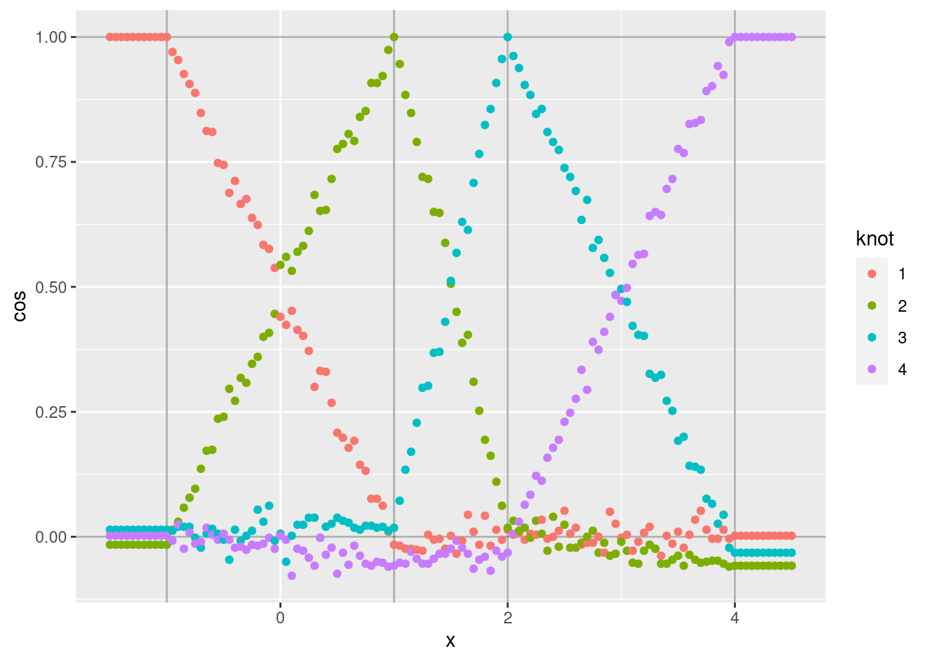

Version	Author	Date
e19cb7e	Ross Gayler	2021-08-16

Each curve shows the cosine similarity of the encoded scalar (\(x\)) to the VSA vector corresponding to one of the knots.

Each curve shows the expected linear ramp as it moves between the two bounding knots.
The cosine similarity at the peak of each curve is exactly one because the encoded scalar is identical to the corresponding knot vector.
The curves corresponding to intermediate values of \(x\) are noisy around a straight line. The noise is due to the encoding being a random weighted blend of the bounding knot vectors (due to applying vsa_add()).
The minimum values of each curve are not exactly zero, because they correspond to the angle between two randomly selected vectors. That is, the cosine similarity is distributed around zero. Repeat that analysis using relatively high dimensional VSA vectors (vsa_dim = 1e5) to reduce the variability of the results.

# make an encoder specification with realistic vector dimension
ss <- vsa_mk_scalar_encoder_spline_spec(vsa_dim = 1e5L, knots = c(-1, 1, 2, 4))

# get the vectors corresponding to the knots
v1 <- ss$knots_vsa[[1]]
v2 <- ss$knots_vsa[[2]]
v3 <- ss$knots_vsa[[3]]
v4 <- ss$knots_vsa[[4]]

# make a sequence of scalar values that (more than) span the knot range
d <- tibble::tibble(
  x = seq(from = -1.5, to = 4.5, by = 0.05)
) %>% 
  dplyr::rowwise() %>% 
  dplyr::mutate(
    # encode each value of x
    v_x = vsa_encode_scalar_spline(x[[1]], ss) %>% list(),
    # get the cosine between the encoded x and each of the knot vectors
    cos_1 = vsa_cos_sim(v_x, v1),
    cos_2 = vsa_cos_sim(v_x, v2),
    cos_3 = vsa_cos_sim(v_x, v3),
    cos_4 = vsa_cos_sim(v_x, v4)
  ) %>% 
  dplyr::ungroup() %>%
  dplyr::select(-v_x) %>% 
  tidyr::pivot_longer(cos_1:cos_4, 
                      names_to = "knot", names_prefix = "cos_", 
                      values_to = "cos")

d %>% ggplot(aes(x = x)) +
  geom_hline(yintercept = c(0, 1), alpha = 0.3) +
  geom_vline(xintercept = c(-1, 1, 2, 4), alpha = 0.3) +
  geom_point(aes(y = cos, colour = knot))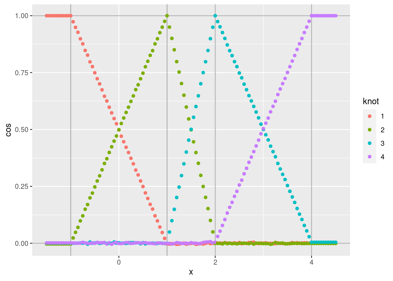

Version	Author	Date
e19cb7e	Ross Gayler	2021-08-16

As expected, the noise is greatly reduced.

With the linear spline encoding, the representations at the knots are always identical to the knot vectors. For intermediate values of the numeric scalar the encoding is a weighted blend of the bounding knot vectors. This blending is implemented by vsa_add(), so the encoding will be different on each occasion the encoding is generated.

Demonstrate the distribution of cosine similarity between encodings of the same scalar value. Use a scalar value midway between the bounding knots to maximise the variation between encodings.

Use VSA vectors with dimensionality \(10^4\) to match the default dimensionality we intend to use.

# make an encoder specification with realistic vector dimension
ss <- vsa_mk_scalar_encoder_spline_spec(vsa_dim = 1e4L, knots = c(0, 1))

# generate n pairs of encodings of the same scalar (x)
x <- 0.5 # scalar to encode (in the range 0 .. 1)
n <- 1e3 # number of pairs to create
# make a one-column data frame with the cos similarity of each vector pair
d <- tibble::tibble(
  cos = purrr::map_dbl(1:n, ~ 
                         vsa_cos_sim(
                           vsa_encode_scalar_spline(x, ss), 
                           vsa_encode_scalar_spline(x, ss)
                         )
  )
) 

d %>% ggplot() +
  geom_histogram(aes(x = cos))

`stat_bin()` using `bins = 30`. Pick better value with `binwidth`.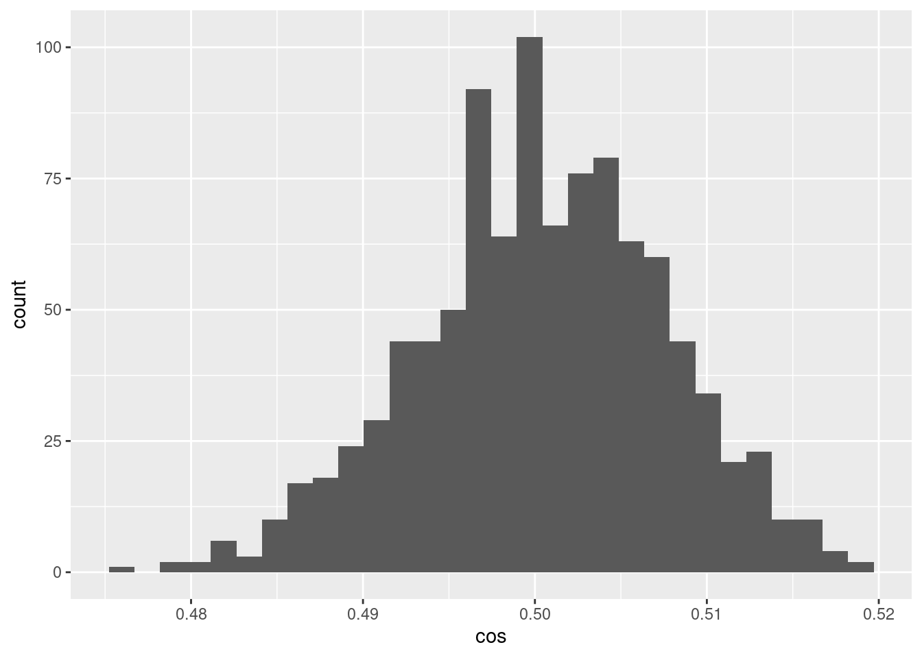

Version	Author	Date
e19cb7e	Ross Gayler	2021-08-16

The encoded values of the scalar midway between the bounding knots differ randomly and have a distribution of cosine similarities to each other that are fairly tightly bounded around 0.5

Repeat the analysis for a scalar much nearer one of the knots.

# make an encoder specification with realistic vector dimension
ss <- vsa_mk_scalar_encoder_spline_spec(vsa_dim = 1e4L, knots = c(0, 1))

# generate n pairs of encodings of the same scalar (x)
x <- 0.05 # scalar to encode (in the range 0 .. 1)
n <- 1e3 # number of pairs to create
# make a one-column data frame with the cos similarity of each vector pair
d <- tibble::tibble(
  cos = purrr::map_dbl(1:n, ~ 
                         vsa_cos_sim(
                           vsa_encode_scalar_spline(x, ss), 
                           vsa_encode_scalar_spline(x, ss)
                         )
  )
) 

d %>% ggplot() +
  geom_histogram(aes(x = cos))

`stat_bin()` using `bins = 30`. Pick better value with `binwidth`.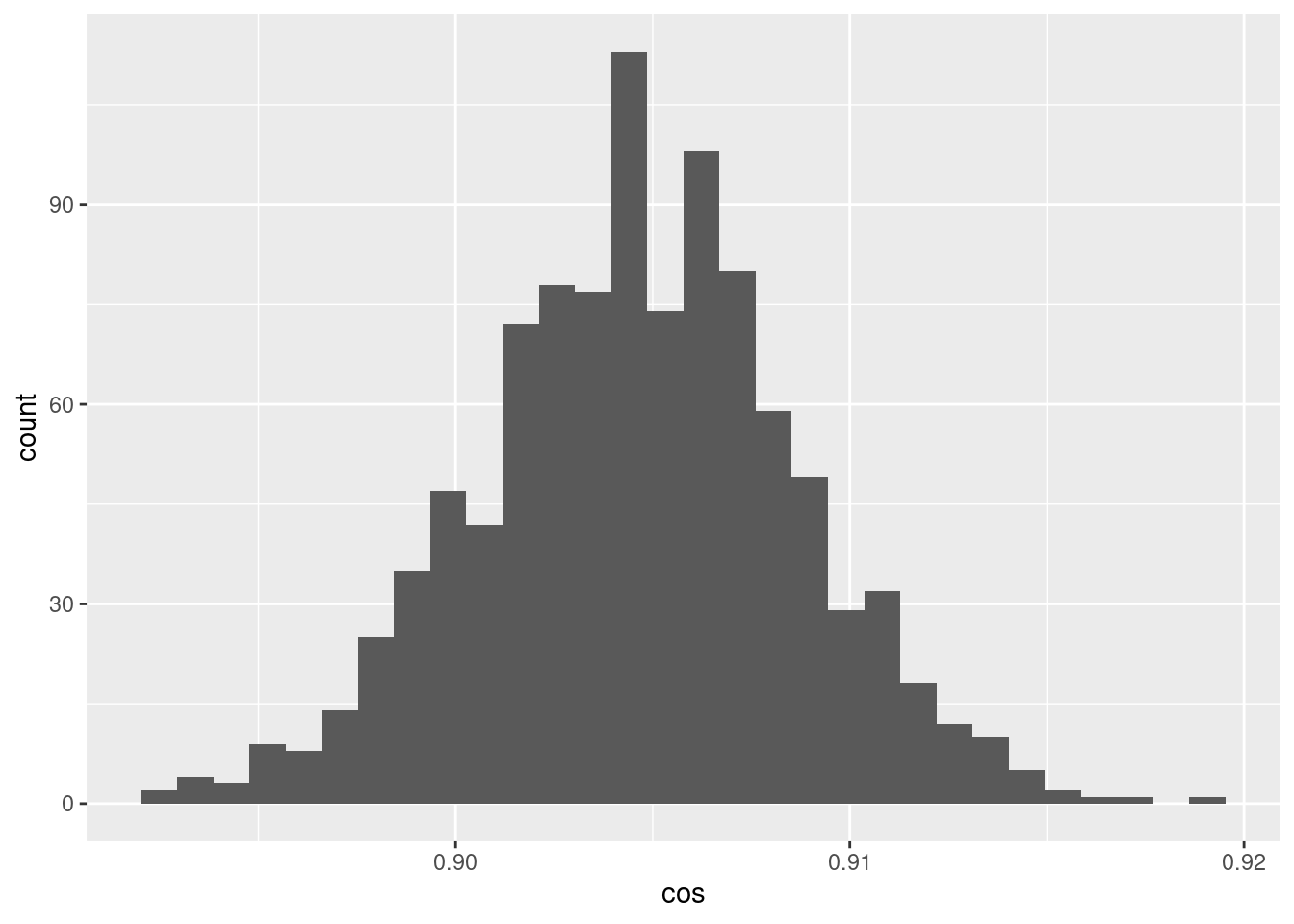

Version	Author	Date
e19cb7e	Ross Gayler	2021-08-16

The cosine similarities between pairs of encodings of the scalar 0.05 is a much tighter distribution around ~0.905

The fact that the encoding is constant at the knots and more variable between knots seems rather odd. If this is a problem the encoding could be made constant by using a fixed seed to vsa_add().

sessionInfo()

R version 4.1.1 (2021-08-10)
Platform: x86_64-pc-linux-gnu (64-bit)
Running under: Ubuntu 21.04

Matrix products: default
BLAS:   /usr/lib/x86_64-linux-gnu/blas/libblas.so.3.9.0
LAPACK: /usr/lib/x86_64-linux-gnu/lapack/liblapack.so.3.9.0

locale:
 [1] LC_CTYPE=en_AU.UTF-8       LC_NUMERIC=C              
 [3] LC_TIME=en_AU.UTF-8        LC_COLLATE=en_AU.UTF-8    
 [5] LC_MONETARY=en_AU.UTF-8    LC_MESSAGES=en_AU.UTF-8   
 [7] LC_PAPER=en_AU.UTF-8       LC_NAME=C                 
 [9] LC_ADDRESS=C               LC_TELEPHONE=C            
[11] LC_MEASUREMENT=en_AU.UTF-8 LC_IDENTIFICATION=C       

attached base packages:
[1] stats     graphics  grDevices datasets  utils     methods   base     

other attached packages:
[1] tibble_3.1.3       Matrix_1.3-4       dplyr_1.0.7        DiagrammeR_1.0.6.1
[5] ggplot2_3.3.5      purrr_0.3.4        magrittr_2.0.1     here_1.0.1        

loaded via a namespace (and not attached):
 [1] Rcpp_1.0.7         highr_0.9          RColorBrewer_1.1-2 pillar_1.6.2      
 [5] compiler_4.1.1     later_1.2.0        git2r_0.28.0       workflowr_1.6.2   
 [9] tools_4.1.1        digest_0.6.27      lattice_0.20-44    jsonlite_1.7.2    
[13] evaluate_0.14      lifecycle_1.0.0    gtable_0.3.0       pkgconfig_2.0.3   
[17] rlang_0.4.11       rstudioapi_0.13    cli_3.0.1          yaml_2.2.1        
[21] xfun_0.25          withr_2.4.2        stringr_1.4.0      knitr_1.33        
[25] htmlwidgets_1.5.3  generics_0.1.0     fs_1.5.0           vctrs_0.3.8       
[29] tidyselect_1.1.1   rprojroot_2.0.2    grid_4.1.1         glue_1.4.2        
[33] R6_2.5.0           fansi_0.5.0        rmarkdown_2.10     bookdown_0.22     
[37] farver_2.1.0       tidyr_1.1.3        whisker_0.4        scales_1.1.1      
[41] promises_1.2.0.1   ellipsis_0.3.2     htmltools_0.5.1.1  colorspace_2.0-2  
[45] renv_0.14.0        httpuv_1.6.1       labeling_0.4.2     utf8_1.2.2        
[49] stringi_1.7.3      visNetwork_2.0.9   munsell_0.5.0      crayon_1.4.1

Scalar Encoder/Decoder (Linear Interpolation Spline)

Ross Gayler

2021-08-12

1 Make encoder specification

2 Apply encoding