PID Task Analysis
Ross Gayler
2021-08-20
Last updated: 2021-08-20
Checks: 7 0
Knit directory:
VSA_altitude_hold/
This reproducible R Markdown analysis was created with workflowr (version 1.6.2). The Checks tab describes the reproducibility checks that were applied when the results were created. The Past versions tab lists the development history.
Great! Since the R Markdown file has been committed to the Git repository, you know the exact version of the code that produced these results.
Great job! The global environment was empty. Objects defined in the global environment can affect the analysis in your R Markdown file in unknown ways. For reproduciblity it’s best to always run the code in an empty environment.
The command set.seed(20210617) was run prior to running the code in the R Markdown file.
Setting a seed ensures that any results that rely on randomness, e.g.
subsampling or permutations, are reproducible.
Great job! Recording the operating system, R version, and package versions is critical for reproducibility.
Nice! There were no cached chunks for this analysis, so you can be confident that you successfully produced the results during this run.
Great job! Using relative paths to the files within your workflowr project makes it easier to run your code on other machines.
Great! You are using Git for version control. Tracking code development and connecting the code version to the results is critical for reproducibility.
The results in this page were generated with repository version 415989a. See the Past versions tab to see a history of the changes made to the R Markdown and HTML files.
Note that you need to be careful to ensure that all relevant files for the
analysis have been committed to Git prior to generating the results (you can
use wflow_publish or wflow_git_commit). workflowr only
checks the R Markdown file, but you know if there are other scripts or data
files that it depends on. Below is the status of the Git repository when the
results were generated:
Ignored files:
    Ignored:    .Rhistory
    Ignored:    .Rproj.user/
    Ignored:    renv/library/
    Ignored:    renv/local/
    Ignored:    renv/staging/
Note that any generated files, e.g. HTML, png, CSS, etc., are not included in this status report because it is ok for generated content to have uncommitted changes.
These are the previous versions of the repository in which changes were made
to the R Markdown (analysis/PID_task_analysis.Rmd) and HTML (docs/PID_task_analysis.html)
files. If you’ve configured a remote Git repository (see
?wflow_git_remote), click on the hyperlinks in the table below to
view the files as they were in that past version.
| File | Version | Author | Date | Message |
|---|---|---|---|---|
| Rmd | 415989a | Ross Gayler | 2021-08-20 | WIP |
| html | 415989a | Ross Gayler | 2021-08-20 | WIP |
| html | de8dbda | Ross Gayler | 2021-08-18 | Build site. |
| Rmd | af002d9 | Ross Gayler | 2021-08-18 | Add linear spline scalar encoder |
This notebook attempts to statistically characterise the PID controller as a black-box function.
Looking at the data flow diagram for Design 01, and ignoring the tuning parameters, there are three input variables:
- Altitude (\(z\))
- Vertical velocity (\(dz\))
- Target altitude (\(k_{tgt}\))
And one output variable:
- Clipped motor demand (\(i8 \triangleq u\))
The integrated error nodes (\(i4\), \(i5\), \(i9\)) introduce a history dependence into the PID function. This part of the DFD implements the “I” (integral) term of “PID” controller. However, the previous analyses of the simulation data suggest that the integral term is only effective in the final phase of the approach to the target altitude, and introduces an (at best) harmless oscillation. This suggests that the I term may be unnecessary in this application.
If the I (integrated error) term is dropped from the PID controller it becomes a purely feedforward, stateless function, which would be very easy to implement.
The purpose of this notebook is to statistically characterise the PID controller function as a stateless, feedforward function. This function could be compared to the simulated data to see what has been lost by dropping the I term.
It is worth emphasizing that the PID controller being modelled is completely fixed (i.e.it does not learn the control function and is not adaptive to any changes) and is not guarnteed to be optimally tuned.
1 Read data
This notebook is based on the data generated by the simulation runs with multiple target altitudes per run.
Read the data from the simulations and mathematically reconstruct the values of the nodes not included in the input files.
# function to clip value to a range
clip <- function(
  x, # numeric
  x_min, # numeric[1] - minimum output value
  x_max  # numeric[1] - maximum output value
) # value # numeric - x constrained to the range [x_min, x_max]
  {
  x %>% pmax(x_min) %>% pmin(x_max)
}

# function to extract a numeric parameter value from the file name
get_param_num <- function(
  file, # character - vector of file names
  regexp # character[1] - regular expression for "param=value"
         # use a capture group to get the value part
) # value # numeric - vector of parameter values
{
  file %>% str_match(regexp) %>%
      subset(select = 2) %>% as.numeric()
}

# function to extract a sequence of numeric parameter values from the file name
get_param_num_seq <- function(
  file, # character - vector of file names
  regexp # character[1] - regular expression for "param=value"
         # use a capture group to get the value part
) # value # character - character representation of a sequence, e.g. "(1,2,3)"
{
  file %>% str_match(regexp) %>%
      subset(select = 2) %>%
    str_replace_all(c("^" = "(", "_" = ",", "$" = ")")) # reformat as sequence
}

# function to extract a logical parameter value from the file name
get_param_log <- function(
  file, # character - vector of file names
  regexp # character[1] - regular expression for "param=value"
  # use a capture group to get the value part
  # value *must* be T or F
) # value # logical - vector of logical parameter values
{
  file %>% str_match(regexp) %>%
    subset(select = 2) %>% as.character() %>% "=="("T")
}

# read the data
d_wide <- fs::dir_ls(path = here::here("data", "multiple_target"), regexp = "/targets=.*\\.csv$") %>% # get file paths
  vroom::vroom(id = "file") %>% # read files
  dplyr::rename(k_tgt = target) %>% # rename for consistency with single target data
  dplyr::mutate( # add extra columns
    file = file %>% fs::path_ext_remove() %>% fs::path_file(), # get file name
    # get parameters
    targets  = file %>% get_param_num_seq("targets=([._0-9]+)_start="), # hacky
    k_start  = file %>% get_param_num("start=([.0-9]+)"),
    sim_id   = paste(targets, k_start), # short ID for each simulation
    k_p      = file %>% get_param_num("kp=([.0-9]+)"),
    k_i      = file %>% get_param_num("Ki=([.0-9]+)"),
    # k_tgt    = file %>% get_param_num("k_tgt=([.0-9]+)"), # no longer needed
    k_windup = file %>% get_param_num("k_windup=([.0-9]+)"),
    uclip    = FALSE, # constant across all files
    dz0      = TRUE, # constant across all files
    # Deal with the fact that the interpretation of the imported u value
    # depends on the uclip parameter
    u_import = u, # keep a copy of the imported value to one side
    u = dplyr::if_else(uclip, # make u the "correct" value
                       u_import,
                       clip(u_import, 0, 1)
                       ),
    # reconstruct the missing nodes
    i1 = k_tgt - z,
    i2 = i1 - dz,
    i3 = e * k_p,
    i9 = lag(ei, n = 1, default = 0), # initialised to zero
    i4 = e + i9,
    i5 = i4 %>% clip(-k_windup, k_windup),
    i6 = ei * k_i,
    i7 = i3 + i6,
    i8 = i7 %>% clip(0, 1)
  ) %>%
  # add time variable per file
  dplyr::group_by(file) %>%
  dplyr::mutate(t = 1:n()) %>%
  dplyr::ungroup()
Rows: 6000 Columns: 8── Column specification ────────────────────────────────────────────────────────
Delimiter: ","
dbl (7): time, target, z, dz, e, ei, u
ℹ Use `spec()` to retrieve the full column specification for this data.
ℹ Specify the column types or set `show_col_types = FALSE` to quiet this message.dplyr::glimpse(d_wide)Rows: 6,000
Columns: 27
$ file <chr> "targets=1_3_5_start=3_kp=0.20_Ki=3.00_k_windup=0.20", "targe…
$ time <dbl> 0.00, 0.01, 0.02, 0.03, 0.04, 0.05, 0.06, 0.07, 0.08, 0.09, 0…
$ k_tgt <dbl> 1, 1, 1, 1, 1, 1, 1, 1, 1, 1, 1, 1, 1, 1, 1, 1, 1, 1, 1, 1, 1…
$ z <dbl> 3.000, 3.000, 3.003, 3.005, 3.006, 3.006, 3.005, 3.002, 2.999…
$ dz <dbl> 0.000, 0.286, 0.188, 0.090, -0.008, -0.106, -0.204, -0.302, -…
$ e <dbl> -2.000, -2.286, -2.191, -2.095, -1.998, -1.899, -1.800, -1.70…
$ ei <dbl> -0.200, -0.200, -0.200, -0.200, -0.200, -0.200, -0.200, -0.20…
$ u <dbl> 0.000, 0.000, 0.000, 0.000, 0.000, 0.000, 0.000, 0.000, 0.000…
$ targets <chr> "(1,3,5)", "(1,3,5)", "(1,3,5)", "(1,3,5)", "(1,3,5)", "(1,3,…
$ k_start <dbl> 3, 3, 3, 3, 3, 3, 3, 3, 3, 3, 3, 3, 3, 3, 3, 3, 3, 3, 3, 3, 3…
$ sim_id <chr> "(1,3,5) 3", "(1,3,5) 3", "(1,3,5) 3", "(1,3,5) 3", "(1,3,5) …
$ k_p <dbl> 0.2, 0.2, 0.2, 0.2, 0.2, 0.2, 0.2, 0.2, 0.2, 0.2, 0.2, 0.2, 0…
$ k_i <dbl> 3, 3, 3, 3, 3, 3, 3, 3, 3, 3, 3, 3, 3, 3, 3, 3, 3, 3, 3, 3, 3…
$ k_windup <dbl> 0.2, 0.2, 0.2, 0.2, 0.2, 0.2, 0.2, 0.2, 0.2, 0.2, 0.2, 0.2, 0…
$ uclip <lgl> FALSE, FALSE, FALSE, FALSE, FALSE, FALSE, FALSE, FALSE, FALSE…
$ dz0 <lgl> TRUE, TRUE, TRUE, TRUE, TRUE, TRUE, TRUE, TRUE, TRUE, TRUE, T…
$ u_import <dbl> -1.000, -1.057, -1.038, -1.019, -1.000, -0.980, -0.960, -0.94…
$ i1 <dbl> -2.000, -2.000, -2.003, -2.005, -2.006, -2.006, -2.005, -2.00…
$ i2 <dbl> -2.000, -2.286, -2.191, -2.095, -1.998, -1.900, -1.801, -1.70…
$ i3 <dbl> -0.4000, -0.4572, -0.4382, -0.4190, -0.3996, -0.3798, -0.3600…
$ i9 <dbl> 0.000, -0.200, -0.200, -0.200, -0.200, -0.200, -0.200, -0.200…
$ i4 <dbl> -2.000, -2.486, -2.391, -2.295, -2.198, -2.099, -2.000, -1.90…
$ i5 <dbl> -0.200, -0.200, -0.200, -0.200, -0.200, -0.200, -0.200, -0.20…
$ i6 <dbl> -0.600, -0.600, -0.600, -0.600, -0.600, -0.600, -0.600, -0.60…
$ i7 <dbl> -1.0000, -1.0572, -1.0382, -1.0190, -0.9996, -0.9798, -0.9600…
$ i8 <dbl> 0.0000, 0.0000, 0.0000, 0.0000, 0.0000, 0.0000, 0.0000, 0.000…
$ t <int> 1, 2, 3, 4, 5, 6, 7, 8, 9, 10, 11, 12, 13, 14, 15, 16, 17, 18…1.1 Plot the data
The altitude error (\(i1\)) is a deterministic function of the altitude (\(z\)) and the altitude target (\(k_{tgt}\)). The two inputs \(z\) and \(k_{tgt}\) can be replaced with the single input \(i1\). This has the advantage of meaning that there are only two inputs \(i1\), and \(dz\), which can be represented on a plane.
Display the distribution of input values to the PID controller across all simulation runs.
d_wide %>%
  ggplot(aes(x = i1, y = dz)) +
  geom_point(alpha = 0.1)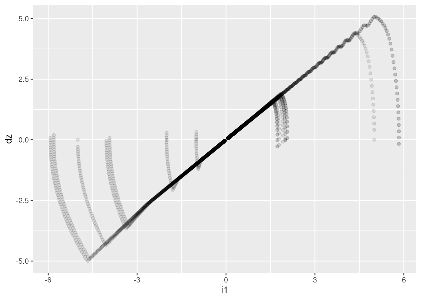
- The dark (because there are many overlapping points) diagonal line corresponds to the final phase of all the trajectories where the altitude error and vertical velocity both decrease to zero with any approximately constant ratio between the two quantities.
- The light, approximately vertical curves correspond to the initial phase of all the trajectories, where the multicopter is either climbing at full power or dropping at zero power.
Add the clipped motor command to the plot.
The clipped motor command lies in the range \([0, 1]\) and 0.524 is the command level for hovering. It will be useful to rescale the motor command level so that zero corresponds to hover and the magnitude of the maximum deviation from hover is one.
p <- d_wide %>%
  dplyr::mutate(i8_scl = (i8 - 0.524) / 0.524) %>%
  ggplot(aes(group = paste(sim_id, k_tgt))) +
  scale_color_viridis_c()

p +
  geom_abline(slope = 1, intercept = 0, colour = "red") +
  geom_point(aes(x = i1, y = dz,
                 size = abs(i8_scl), colour = i8_scl),
             alpha = 0.5) +
  geom_path(aes(x = i1, y = dz), alpha = 0.2)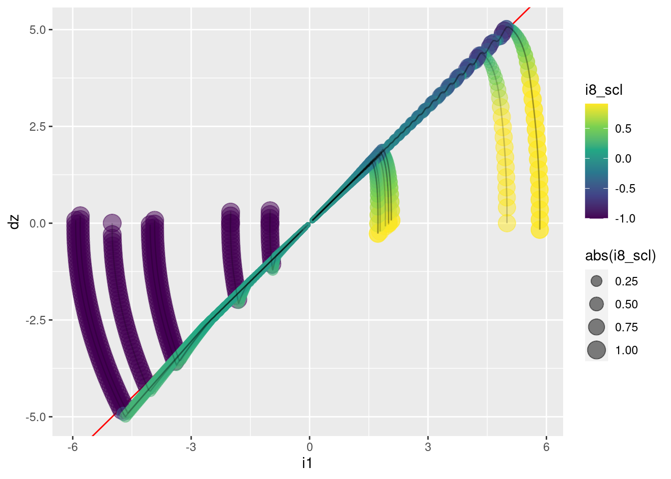
p +
  geom_point(aes(x = i1, y = i8_scl,
                 size = abs(i8_scl), colour = i8_scl),
             alpha = 0.5) +
  geom_path(aes(x = i1, y = i8_scl), alpha = 0.2)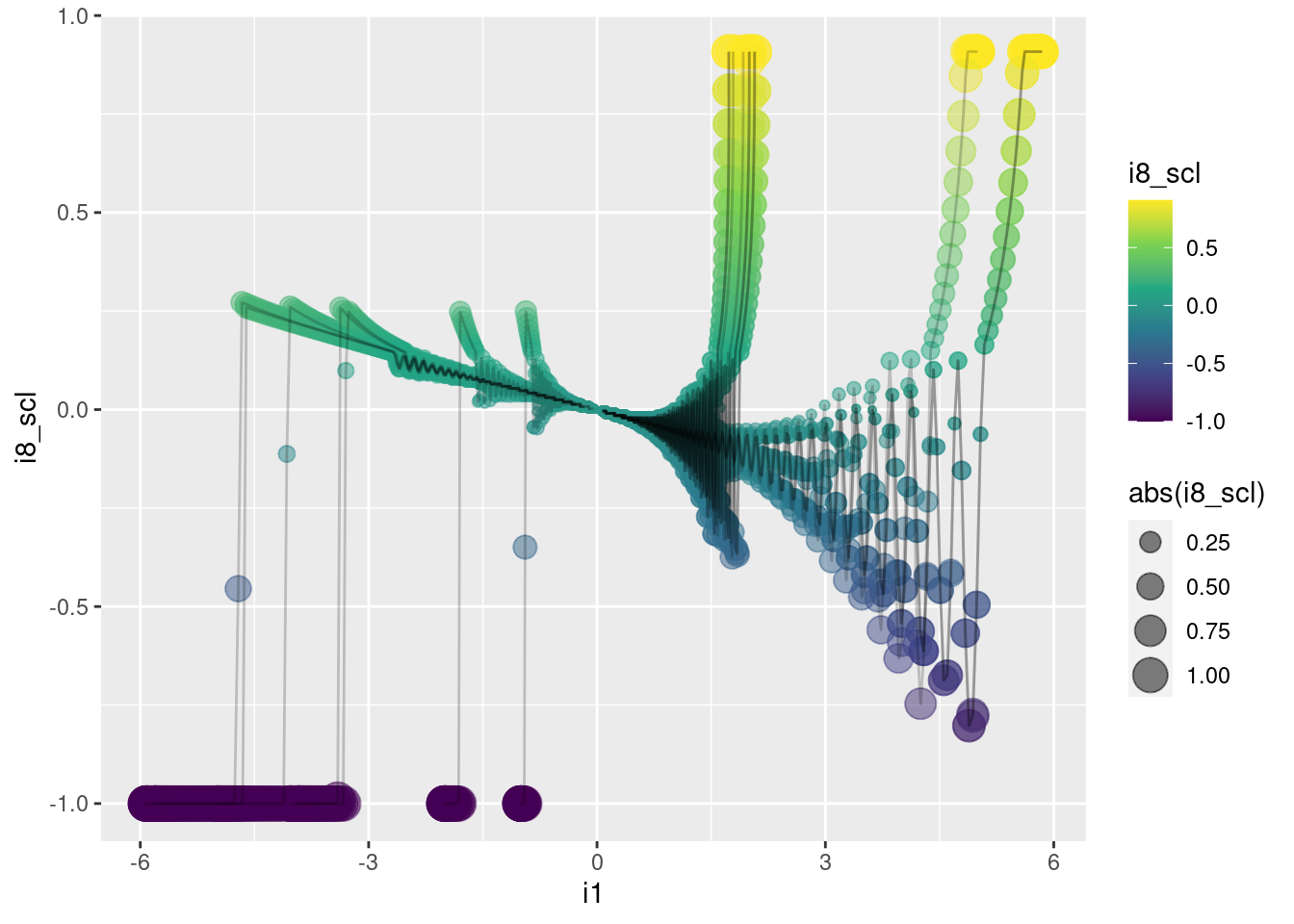
p +
  geom_point(aes(x = dz, y = i8_scl,
                 size = abs(i8_scl), colour = i8_scl),
             alpha = 0.5) +
  geom_path(aes(x = dz, y = i8_scl), alpha = 0.2)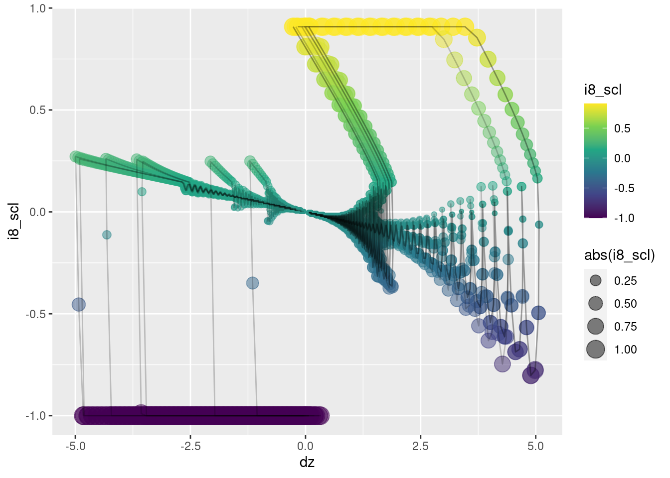
Repeat that with the unclipped motor command (\(i7\)).
p <- d_wide %>%
  dplyr::mutate(i7_scl = (i7 - 0.524) / 0.524) %>%
  ggplot(aes(group = paste(sim_id, k_tgt))) +
  scale_color_viridis_c()

p +
  geom_abline(slope = 1, intercept = 0, colour = "red") +
  geom_point(aes(x = i1, y = dz,
                 size = abs(i7_scl), colour = i7_scl),
             alpha = 0.5) +
  geom_path(aes(x = i1, y = dz), alpha = 0.2)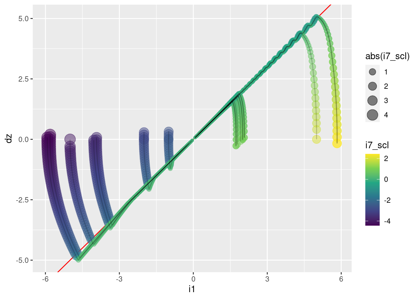
p +
  geom_point(aes(x = i1, y = i7_scl,
                 size = abs(i7_scl), colour = i7_scl),
             alpha = 0.5) +
  geom_path(aes(x = i1, y = i7_scl), alpha = 0.2)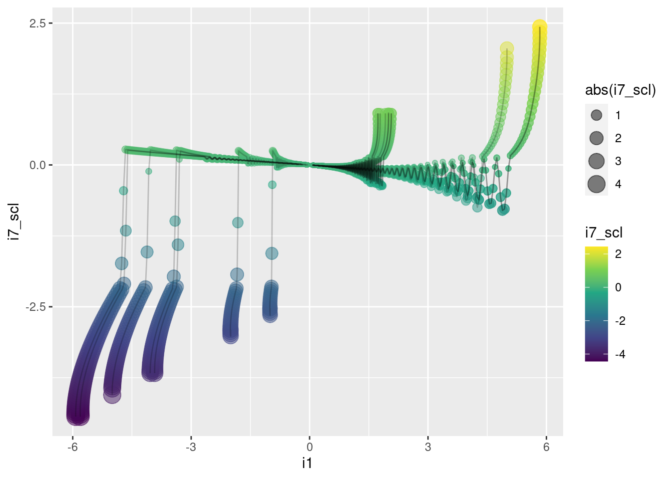
p +
  geom_point(aes(x = dz, y = i7_scl,
                 size = abs(i7_scl), colour = i7_scl),
             alpha = 0.5) +
  geom_path(aes(x = dz, y = i7_scl), alpha = 0.2)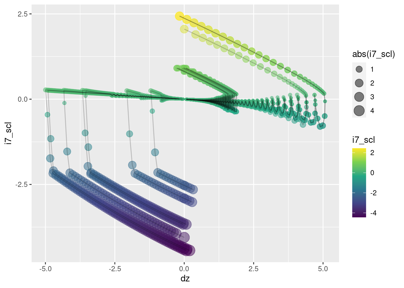
sessionInfo()R version 4.1.1 (2021-08-10)
Platform: x86_64-pc-linux-gnu (64-bit)
Running under: Ubuntu 21.04
Matrix products: default
BLAS: /usr/lib/x86_64-linux-gnu/blas/libblas.so.3.9.0
LAPACK: /usr/lib/x86_64-linux-gnu/lapack/liblapack.so.3.9.0
locale:
[1] LC_CTYPE=en_AU.UTF-8 LC_NUMERIC=C
[3] LC_TIME=en_AU.UTF-8 LC_COLLATE=en_AU.UTF-8
[5] LC_MONETARY=en_AU.UTF-8 LC_MESSAGES=en_AU.UTF-8
[7] LC_PAPER=en_AU.UTF-8 LC_NAME=C
[9] LC_ADDRESS=C LC_TELEPHONE=C
[11] LC_MEASUREMENT=en_AU.UTF-8 LC_IDENTIFICATION=C
attached base packages:
[1] stats graphics grDevices datasets utils methods base
other attached packages:
[1] tibble_3.1.3 Matrix_1.3-4 purrr_0.3.4 DiagrammeR_1.0.6.1
[5] ggplot2_3.3.5 stringr_1.4.0 dplyr_1.0.7 vroom_1.5.4
[9] here_1.0.1 fs_1.5.0
loaded via a namespace (and not attached):
[1] tidyselect_1.1.1 xfun_0.25 lattice_0.20-44 colorspace_2.0-2
[5] vctrs_0.3.8 generics_0.1.0 viridisLite_0.4.0 htmltools_0.5.1.1
[9] yaml_2.2.1 utf8_1.2.2 rlang_0.4.11 later_1.3.0
[13] pillar_1.6.2 glue_1.4.2 withr_2.4.2 bit64_4.0.5
[17] RColorBrewer_1.1-2 lifecycle_1.0.0 munsell_0.5.0 gtable_0.3.0
[21] workflowr_1.6.2 visNetwork_2.0.9 htmlwidgets_1.5.3 evaluate_0.14
[25] labeling_0.4.2 knitr_1.33 tzdb_0.1.2 httpuv_1.6.2
[29] parallel_4.1.1 fansi_0.5.0 highr_0.9 Rcpp_1.0.7
[33] renv_0.14.0 promises_1.2.0.1 scales_1.1.1 jsonlite_1.7.2
[37] farver_2.1.0 bit_4.0.4 digest_0.6.27 stringi_1.7.3
[41] bookdown_0.23 rprojroot_2.0.2 grid_4.1.1 cli_3.0.1
[45] tools_4.1.1 magrittr_2.0.1 crayon_1.4.1 whisker_0.4
[49] pkgconfig_2.0.3 ellipsis_0.3.2 rmarkdown_2.10 rstudioapi_0.13
[53] R6_2.5.0 git2r_0.28.0 compiler_4.1.1