01-3_check_resid
Check residence variables
Ross Gayler
2021-01-12
Last updated: 2021-01-15
Checks: 7 0
Knit directory:
fa_sim_cal/
This reproducible R Markdown analysis was created with workflowr (version 1.6.2). The Checks tab describes the reproducibility checks that were applied when the results were created. The Past versions tab lists the development history.
Great! Since the R Markdown file has been committed to the Git repository, you know the exact version of the code that produced these results.
Great job! The global environment was empty. Objects defined in the global environment can affect the analysis in your R Markdown file in unknown ways. For reproduciblity it’s best to always run the code in an empty environment.
The command set.seed(20201104) was run prior to running the code in the R Markdown file.
Setting a seed ensures that any results that rely on randomness, e.g.
subsampling or permutations, are reproducible.
Great job! Recording the operating system, R version, and package versions is critical for reproducibility.
Nice! There were no cached chunks for this analysis, so you can be confident that you successfully produced the results during this run.
Great job! Using relative paths to the files within your workflowr project makes it easier to run your code on other machines.
Great! You are using Git for version control. Tracking code development and connecting the code version to the results is critical for reproducibility.
The results in this page were generated with repository version af08f78. See the Past versions tab to see a history of the changes made to the R Markdown and HTML files.
Note that you need to be careful to ensure that all relevant files for the
analysis have been committed to Git prior to generating the results (you can
use wflow_publish or wflow_git_commit). workflowr only
checks the R Markdown file, but you know if there are other scripts or data
files that it depends on. Below is the status of the Git repository when the
results were generated:
Ignored files:
    Ignored:    .Rhistory
    Ignored:    .Rproj.user/
    Ignored:    .tresorit/
    Ignored:    data/VR_20051125.txt.xz
    Ignored:    output/ent_cln.fst
    Ignored:    output/ent_raw.fst
    Ignored:    renv/library/
    Ignored:    renv/staging/
Note that any generated files, e.g. HTML, png, CSS, etc., are not included in this status report because it is ok for generated content to have uncommitted changes.
These are the previous versions of the repository in which changes were made
to the R Markdown (analysis/01-3_check_resid.Rmd) and HTML (docs/01-3_check_resid.html)
files. If you’ve configured a remote Git repository (see
?wflow_git_remote), click on the hyperlinks in the table below to
view the files as they were in that past version.
| File | Version | Author | Date | Message |
|---|---|---|---|---|
| Rmd | c674a51 | Ross Gayler | 2021-01-15 | Add 01-6 clean vars |
| html | cb9bf70 | Ross Gayler | 2021-01-12 | Build site. |
| Rmd | 84d53a0 | Ross Gayler | 2021-01-12 | Add 01-3 check resid |
# Set up the project environment, because each Rmd file knits in a new R session
# so doesn't get the project setup from .Rprofile

# Project setup
library(here)
source(here::here("code", "setup_project.R"))
── Attaching packages ─────────────────────────────────────── tidyverse 1.3.0 ──✓ ggplot2 3.3.3 ✓ purrr 0.3.4
✓ tibble 3.0.4 ✓ dplyr 1.0.2
✓ tidyr 1.1.2 ✓ stringr 1.4.0
✓ readr 1.4.0 ✓ forcats 0.5.0── Conflicts ────────────────────────────────────────── tidyverse_conflicts() ──
x dplyr::filter() masks stats::filter()
x dplyr::lag() masks stats::lag()# Extra set up for the 01*.Rmd notebooks
source(here::here("code", "setup_01.R"))
Attaching package: 'glue'The following object is masked from 'package:dplyr':
collapse# Extra set up for this notebook
# ???
# start the execution time clock
tictoc::tic("Computation time (excl. render)")1 Introduction
The 01*.Rmd notebooks read the data, filter it to the subset to be
used for modelling, characterise it to understand it, check for possible
gotchas, clean it, and save it for the analyses proper.
This notebook (01-3_check_resid) characterises the residence variables
in the saved subset of the data. These are the residential address and
the phone number (which is tied to the address if the telephone is a
land-line).
We have no intention of using the residence variables as predictors for entity resolution. However, they may be of use for manually checking the results of entity resolution. Consequently, the checking done here is minimal.
Define the residence variables.
vars_resid <- c(
  "unit_num", "house_num",
  "half_code", "street_dir", "street_name", "street_type_cd", "street_sufx_cd",
  "res_city_desc", "state_cd", "zip_code",
  "area_cd", "phone_num"
)
Read the usable data. Remember that this consists of only the ACTIVE & VERIFIED records.
# Show the entity data file location
# This is set in code/file_paths.R
fs::path_file(f_entity_raw_fst)
[1] "ent_raw.fst"# get data for next section of analyses
d <- fst::read_fst(
f_entity_raw_fst,
columns = vars_resid
) %>%
tibble::as_tibble()
dim(d)[1] 4099699 12Look at some examples.
Residential address:
d %>%
  dplyr::select(unit_num : zip_code) %>%
  dplyr::slice_sample(n = 20) %>%
knitr::kable()| unit_num | house_num | half_code | street_dir | street_name | street_type_cd | street_sufx_cd | res_city_desc | state_cd | zip_code |
|---|---|---|---|---|---|---|---|---|---|
| NA | 2883 | NA | NA | EASY | ST | NA | DUNN | NC | 28334 |
| NA | 665 | NA | NA | MOUNT OLIVE CHURCH | RD | NA | FRANKLINTON | NC | 27525 |
| NA | 417 | NA | NA | EDINBURGH | DR | NA | FAYETTEVILLE | NC | 28303 |
| NA | 2517 | NA | NA | KERR | AVE | N | WILMINGTON | NC | 28405 |
| NA | 2337 | NA | NA | CLEVELAND | AVE | NA | FAYETTEVILLE | NC | 28312 |
| NA | 9435 | NA | NA | NC HWY 87 | NA | N | PITTSBORO | NC | 27312 |
| NA | 215 | NA | NA | ORANGE | ST | NA | ROCKY MOUNT | NC | 27801 |
| A317 | 733 | NA | NA | PLANTATION ESTATES | DR | NA | MATTHEWS | NC | 28105 |
| 2 | 5311 | NA | NA | 25 70 | HWY | NA | MARSHALL | NC | 28753 |
| NA | 424 | NA | N | KING | ST | NA | ST PAULS | NC | 28384 |
| NA | 13429 | NA | NA | OLD STAGE | RD | NA | WILLOW SPRINGS | NC | 27592 |
| D | 3247 | NA | NA | CYPRESS PARK | RD | NA | GREENSBORO | NC | 27407 |
| NA | 9925 | NA | NA | PALLISERS | TER | NA | CHARLOTTE | NC | 28210 |
| NA | 114 | NA | NA | GIBBS | RD | NA | NEW BERN | NC | 28560 |
| NA | 8885 | NA | NA | ROCKY RIVER | RD | NA | HARRISBURG | NC | 28075 |
| A | 105 | NA | NA | TAMALPAIS | PT | NA | CHAPEL HILL | NC | 27514 |
| NA | 102 | NA | N | ROXFORD | RD | NA | KINGS MOUNTAIN | NC | 28086 |
| NA | 551 | NA | NA | NICK MCLEAN | RD | NA | BUNNLEVEL | NC | 28323 |
| NA | 2913 | NA | NA | WINDSOR | AVE | NA | CHARLOTTE | NC | 28209 |
| NA | 2200 | NA | NA | GRESHAM LAKE | RD | NA | RALEIGH | NC | 27615 |
Telephone number:
d %>%
  dplyr::select(area_cd : phone_num) %>%
  dplyr::slice_sample(n = 20) %>%
knitr::kable()| area_cd | phone_num |
|---|---|
| 252 | 5364553 |
| 252 | 5235950 |
| NA | NA |
| 828 | 9269783 |
| 910 | 5755969 |
| NA | NA |
| NA | NA |
| NA | NA |
| NA | NA |
| 704 | 8065796 |
| NA | NA |
| 704 | 3920844 |
| NA | NA |
| 828 | 6705254 |
| 252 | 7474543 |
| 252 | 6366840 |
| NA | NA |
| NA | NA |
| NA | NA |
| 910 | 8924300 |
2 Dwelling
unit_num Residential address unit number
house_num Residential address street number
half_code Residential address street number half code
d %>%
  dplyr::select(unit_num, house_num, half_code) %>%
  skimr::skim()
Warning in grepl("^\\s+$", x): input string 13013 is invalid in this localeWarning in grepl("^\\s+$", x): input string 27075 is invalid in this localeWarning in grepl("^\\s+$", x): input string 35910 is invalid in this localeWarning in grepl("^\\s+$", x): input string 40713 is invalid in this localeWarning in grepl("^\\s+$", x): input string 49523 is invalid in this locale| Name | Piped data |
| Number of rows | 4099699 |
| Number of columns | 3 |
| _______________________ | |
| Column type frequency: | |
| character | 3 |
| ________________________ | |
| Group variables | None |
Variable type: character
| skim_variable | n_missing | complete_rate | min | max | empty | n_unique | whitespace |
|---|---|---|---|---|---|---|---|
| unit_num | 3755239 | 0.08 | 1 | 7 | 0 | 16116 | 0 |
| house_num | 0 | 1.00 | 1 | 6 | 0 | 27534 | 0 |
| half_code | 4088996 | 0.00 | 1 | 1 | 0 | 41 | 0 |
unit_num8% filledhouse_num100% filledhalf_code0.3% filled- Warning messages indicate some invalid multibyte strings
Look at half_code.
table(d$half_code, useNA = "ifany")
      -       /       `       +    \xab    \xbd       0       1       2       3
      1       8       5      32       3    1730       1      44      35       5
      4       5       6       7       8       9       A       B       C       D
     10       6       6       5       4       1    3313    2725     948     569
      E       F       G       H       I       J       K       L       M       N
    273     214     154     174      36      78      58      48      48      33
      O       P       Q       R       S       T       U       V       W       X
      6      21       7      13      38      13       3       6      24       4
      Y    <NA>
      1 4088996
d %>%
dplyr::filter(!is.na(half_code)) %>%
dplyr::select(unit_num : street_type_cd) %>%
dplyr::slice_sample(n = 20)# A tibble: 20 x 6
unit_num house_num half_code street_dir street_name street_type_cd
<chr> <chr> <chr> <chr> <chr> <chr>
1 <NA> 640 "\xab" N LOUISIANA AVE
2 <NA> 21 "B" <NA> SPICEWOOD RD
3 <NA> 803 "C" <NA> DOUGLAS DR
4 <NA> 601 "B" W GRAHAM ST
5 <NA> 102 "\xbd" <NA> FAIRWAY DR
6 A 141 "A" <NA> HERRON AVE
7 <NA> 795 "\xbd" <NA> HENDERSONVILLE RD
8 <NA> 1005 "C" <NA> EAST ST
9 <NA> 2840 "D" <NA> ROGERS RD
10 <NA> 717 "C" <NA> DEEP FORD RD
11 <NA> 3211 "A" <NA> BIG WOODS RD
12 <NA> 626 "A" <NA> LUMBEE ST
13 <NA> 910 "D" <NA> CULBRETH AVE
14 <NA> 155 "B" <NA> HIBRITEN MOUNTAIN RD
15 <NA> 901 "B" <NA> OAKLAWN DR
16 <NA> 1314 "A" <NA> BEAVER CREEK SCHOOL RD
17 <NA> 100 "A" <NA> CIRCLE CT
18 <NA> 301 "`" <NA> CHAMPION DR
19 <NA> 21 "B" <NA> MASTERS COURT DR
20 <NA> 114 "D" <NA> SPRUCE HILL LN half_code appears to indicate where there are multiple buildings on
one street-numbered block. Typical values would be A, B, …
3 Street
d %>%
  dplyr::select(starts_with("street_")) %>%
skimr::skim()| Name | Piped data |
| Number of rows | 4099699 |
| Number of columns | 4 |
| _______________________ | |
| Column type frequency: | |
| character | 4 |
| ________________________ | |
| Group variables | None |
Variable type: character
| skim_variable | n_missing | complete_rate | min | max | empty | n_unique | whitespace |
|---|---|---|---|---|---|---|---|
| street_dir | 3812561 | 0.07 | 1 | 2 | 0 | 8 | 0 |
| street_name | 7 | 1.00 | 1 | 30 | 0 | 83244 | 0 |
| street_type_cd | 154594 | 0.96 | 2 | 4 | 0 | 119 | 0 |
| street_sufx_cd | 3941004 | 0.04 | 1 | 3 | 0 | 11 | 0 |
street_dir7% filledstreet_name~100% filled (7 missing)street_type_cd96% filledstreet_sufx_cd4% filled
3.1 street_dir
street_dir Residential address street direction (N,S,E,W,NE,SW, etc.)
table(d$street_dir, useNA = "ifany")
      E       N      NE      NW       S      SE      SW       W    <NA>
  71244   72784    2161     911   68612    1221     729   69476 3812561
3.2 street_name
street_name Residential address street name
Seven records are missing street name. Look at them.
d %>%
  dplyr::filter(is.na(street_name)) %>%
knitr::kable()| unit_num | house_num | half_code | street_dir | street_name | street_type_cd | street_sufx_cd | res_city_desc | state_cd | zip_code | area_cd | phone_num |
|---|---|---|---|---|---|---|---|---|---|---|---|
| NA | 0 | NA | NA | NA | NA | NA | STONY POINT | NC | 28678 | NA | NA |
| NA | 0 | NA | NA | NA | NA | NA | NA | NA | NA | NA | NA |
| NA | 0 | NA | NA | NA | NA | NA | NA | NA | NA | NA | NA |
| NA | 0 | NA | NA | NA | NA | NA | NA | NA | NA | NA | NA |
| NA | 0 | NA | NA | NA | NA | NA | NA | NA | NA | NA | NA |
| NA | 0 | NA | NA | NA | NA | NA | NA | NA | NA | NA | NA |
| NA | 0 | NA | NA | NA | NA | NA | BELMONT | NC | 28012 | NA | NA |
- Seven records have no residential address. Are these homeless people?
Some street names are very short. Look at the distribution of length of street name.
summary(stringr::str_length(d$street_name)) Min. 1st Qu. Median Mean 3rd Qu. Max. NA's
1.00 6.00 8.00 8.78 11.00 30.00 7 d %>%
ggplot() +
geom_histogram(aes(x = stringr::str_length(street_name)), binwidth = 1) +
scale_y_sqrt()Warning: Removed 7 rows containing non-finite values (stat_bin).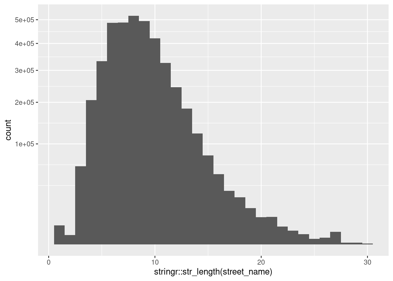
| Version | Author | Date |
|---|---|---|
| cb9bf70 | Ross Gayler | 2021-01-12 |
Look at examples of short street names.
d %>%
  dplyr::filter(stringr::str_length(street_name) == 1) %>%
  dplyr::select(starts_with("street_"), res_city_desc) %>%
  dplyr::slice_sample(n = 20) %>%
knitr::kable()| street_dir | street_name | street_type_cd | street_sufx_cd | res_city_desc |
|---|---|---|---|---|
| NA | C | ST | NA | NEWPORT |
| W | C | ST | NA | ERWIN |
| NA | A | ST | NA | CAMP LEJEUNE |
| E | I | ST | NA | ERWIN |
| NA | F | AVE | NA | KURE BEACH |
| NA | A | ST | NA | LANSING |
| E | K | ST | NA | ERWIN |
| E | C | ST | NA | BUTNER |
| NA | D | ST | NA | SPRING LAKE |
| NA | B | AVE | NA | CHARLOTTE |
| E | B | ST | NA | BUTNER |
| W | B | ST | NA | KANNAPOLIS |
| E | C | ST | NA | BUTNER |
| E | L | ST | NA | ERWIN |
| NA | A | ST | NA | CAMP LEJEUNE |
| NA | E | ST | NA | NORTH WILKESBORO |
| NA | J | AVE | NA | KURE BEACH |
| W | C | ST | NA | BUTNER |
| E | J | ST | NA | MAIDEN |
| NA | E | ST | NA | NORTH WILKESBORO |
d %>%
  dplyr::filter(stringr::str_length(street_name) == 2) %>%
  dplyr::select(starts_with("street_"), res_city_desc) %>%
  dplyr::slice_sample(n = 20) %>%
knitr::kable()| street_dir | street_name | street_type_cd | street_sufx_cd | res_city_desc |
|---|---|---|---|---|
| NA | DJ | DR | NA | BENSON |
| NA | KY | FLDS | NA | WEAVERVILLE |
| NA | 63 | HWY | NA | LEICESTER |
| NA | KY | FLDS | NA | WEAVERVILLE |
| NA | OW | LN | NA | DUNN |
| N | ST | NA | NA | ASHEVILLE |
| NA | KY | FLDS | NA | WEAVERVILLE |
| NA | RH | RD | NA | HICKORY |
| NA | 23 | HWY | NA | MARS HILL |
| NA | DJ | DR | NA | STATESVILLE |
| NA | CY | CIR | NA | CONCORD |
| NA | JR | RD | NA | TIMBERLAKE |
| NA | WR | LN | NA | CLAREMONT |
| NA | 63 | HWY | NA | LEICESTER |
| NA | 19 | HWY | NA | MARS HILL |
| NA | JR | RD | NA | TIMBERLAKE |
| NA | 23 | HWY | NA | MARS HILL |
| NA | AA | DR | NA | TAYLORSVILLE |
| NA | BR | DR | NA | MARION |
| NA | RH | RD | NA | HICKORY |
I checked some of these examples against a map.
- Some streets have names like A, B, C, …
- “JC Road” is a valid street name
Look at examples of long street names.
d %>%
  dplyr::filter(stringr::str_length(street_name) >= 28) %>%
  dplyr::select(starts_with("street_"), res_city_desc) %>%
  dplyr::distinct(.keep_all = TRUE) %>%
  dplyr::arrange(street_name) %>%
knitr::kable()| street_dir | street_name | street_type_cd | street_sufx_cd | res_city_desc |
|---|---|---|---|---|
| NA | BROOKFIELD RETIREMENT CENTER | NA | NA | LILLINGTON |
| NA | CROSS MEMORIAL BAPTIST CHURCH | LOOP | NA | MARION |
| NA | KINGSDALE MANOR NURSING CENTER | NA | NA | LUMBERTON |
| NA | LOMBARDY VILLAGE MOBILE HOME | PARK | NA | LUMBERTON |
| NA | LOMBARDY VILLAGE MOBILE HOME | PARK | NA | SHANNON |
| NA | LOMBARDY VILLAGE MOBILE HOME | PARK | NA | REX |
| NA | NC HWY 197N NEAR COVY ROCK CHU | NA | NA | BURNSVILLE |
| NA | OLD TAMMANY-OINE ROOKER DAIRY | RD | NA | NORLINA |
| NA | SWEPSONVILLE-METHODIST CHURCH | RD | NA | GRAHAM |
| NA | WHEELING VILLAGE TRAILER PARK | NA | NA | WINSTON SALEM |
| NA | WILDLIFE RECREATION AREA ACC | RD | NA | LEXINGTON |
| NA | WISE-FIVE FORKS- ROBERSON FERR | NA | NA | MACON |
Long street names are multi-word phrases
- Some appear to have been truncated
3.3 street_type_cd
street_type_cd Residential address street type (RD, ST, DR, BLVD,
etc.)
table(d$street_type_cd, useNA = "ifany")
    ALY     ANX     ARC     AVE     BCH     BLF    BLVD     BND      BR     BRG
    266      23       7  207808       1      47   27022     250     166       7
    BRK     BTM     BYP     CIR     CLB     CMN    CMNS     COR    COVE    CRES
     56       1    1205   99489      18      28      20      44       3     534
    CRK    CRSE    CRST    CSWY      CT     CTR      CV      DL      DM    DORM
    141       8      12      22  249682      15    2527       4       1    1756
     DR     EST    ESTS    EXPY     EXT    FALL    FLDS     FLS     FLT    FLTS
 926884     457     203      18    4931       2      64      19       8       4
    FRD     FRK    FRST      FT     FWY     GDN    GDNS     GLN     GRN     GRV
      9      13      22       1       4       6     110      61       6      94
    HBR      HL     HLS    HOLW     HTS     HVN     HWY      IS     JCT     KNL
     38     513     261     200    1684      24   44189      19       6     162
   KNLS    LAND     LDG      LK     LKS      LN    LNDG    LOOP     MDW    MDWS
     51       2       6      51      16  347932     371    9505       2      37
   MEWS     MHP     MNR     MTN    ORCH    OVAL    PARK    PASS    PATH    PKWY
    102       2     222      78       7       2    2013     171    1035    6665
     PL     PLZ    PNES    PSGE      PT    RAMP      rd      RD     RDG     ROW
  82253     211      21      21    2263       1       1 1287597    2124     333
    RST     RTE     RUN     SHR    SHRS     SMT     SPG    SPGS    SPUR      SQ
      2    2731    5219       3      33      11       6      32      58    1169
     ST     STA     TER    TPKE    TRAK    TRCE     TRL    TRLR     VIA     VIS
 512983       9    7959      13      10    1319   44565      26       2      60
     VL     VLG     VLY      VW    WALK     WAY    WYND    XING    XRDS    <NA>
      1     991      67     217     581   51625     328     652     163  154594
3.4 street_sufx_cd
street_sufx_cd Residential address street suffix (BUS, EXT, and
directional)
table(d$street_sufx_cd, useNA = "ifany")
    BUS       E     EXT       I       N      NE      NW       S      SE      SW
    169   13021    1481       1   17869   24755   29472   18870   13095   26587
      W    <NA>
  13375 3941004
4 Locality
res_city_desc Residential address city name
state_cd Residential address state code
zip_code Residential address zip code
d %>%
  dplyr::select(res_city_desc : zip_code) %>%
skimr::skim()| Name | Piped data |
| Number of rows | 4099699 |
| Number of columns | 3 |
| _______________________ | |
| Column type frequency: | |
| character | 3 |
| ________________________ | |
| Group variables | None |
Variable type: character
| skim_variable | n_missing | complete_rate | min | max | empty | n_unique | whitespace |
|---|---|---|---|---|---|---|---|
| res_city_desc | 19 | 1 | 3 | 20 | 0 | 783 | 0 |
| state_cd | 18 | 1 | 2 | 2 | 0 | 5 | 0 |
| zip_code | 21 | 1 | 5 | 9 | 0 | 902 | 0 |
res_city_desc~100% filled (19 missing)state_cd~100% filled (19 missing)zip_code~100% filled (19 missing)
Look at the addresses with any missing locality variable.
d %>%
  dplyr::filter(is.na(res_city_desc) | is.na(state_cd) | is.na(zip_code)) %>%
  dplyr::select(house_num : zip_code) %>%
  dplyr::distinct(.keep_all = TRUE) %>%
  dplyr::arrange(state_cd, res_city_desc, zip_code) %>%
knitr::kable()| house_num | half_code | street_dir | street_name | street_type_cd | street_sufx_cd | res_city_desc | state_cd | zip_code |
|---|---|---|---|---|---|---|---|---|
| 5189 | NA | NA | COVE | RD | NA | MARION | NC | NA |
| 5030 | NA | NA | COVE | RD | NA | MARION | NC | NA |
| 0 | NA | NA | H & N MOBILE HOME | PARK | NA | NA | NC | NA |
| 0 | NA | NA | UNKNOWN | NA | NA | NA | NC | NA |
| 1407 | NA | NA | OVERLOOK | DR | NA | LENOIR | NA | 28645 |
| 0 | NA | NA | CONFIDENTIAL | NA | NA | NA | NA | NA |
| 0 | NA | NA | NA | NA | NA | NA | NA | NA |
- Some appear to be good addresses, apart from a missing zip code
- One appears to be a good address, apart from a missing state code
- Some are CONFIDENTIAL addresses, with all details missing
- Some appear to be completely missing the address (homeless persons?)
4.1 state_cd
state_cd Residential address state code
table(d$state_cd, useNA = "ifany")
     GA      NC      SC      TN      VA    <NA>
     13 4099631       1      29       7      18
Residential state codes are almost entirely Georgia
- There are a small number in neighbouring states (non-resident voters?)
4.2 zip_code
zip_code Residential address zip code
The zip codes are not all the same length. Look at the distribution of length of zip code
table(stringr::str_length(d$zip_code), useNA = "ifany")
      5       9    <NA>
4099667      11      21
Look at the 9-digit zip codes.
d %>%
  dplyr::filter(stringr::str_length(zip_code) == 9) %>%
  dplyr::select(street_name : zip_code) %>%
  dplyr::arrange(zip_code) %>%
knitr::kable()| street_name | street_type_cd | street_sufx_cd | res_city_desc | state_cd | zip_code |
|---|---|---|---|---|---|
| ECHO | LN | NA | SANFORD | NC | 273308492 |
| UNKNOWN | NA | NA | LILLINGTON | NC | 275468949 |
| LINCOLN MCKAY | DR | NA | LILLINGTON | NC | 275469001 |
| SMITH | ST | NA | ALBEMARLE | NC | 280014351 |
| INDIAN MOUND | RD | NA | ALBEMARLE | NC | 280019245 |
| POND | ST | NA | ALBEMARLE | NC | 280019766 |
| NC 731 HWY | NA | NA | NORWOOD | NC | 281289420 |
| FRIENDLY MCLEOD | LN | NA | DUNN | NC | 283349250 |
| BEAVER DAM | RD | NA | ERWIN | NC | 283399790 |
| WIRE | RD | NA | LINDEN | NC | 283569413 |
| WALKER | RD | NA | LINDEN | NC | 283569416 |
- 5-digit and 9-digit zip codes are valid
Timing
Computation time (excl. render): 28.174 sec elapsed
sessionInfo()R version 4.0.3 (2020-10-10)
Platform: x86_64-pc-linux-gnu (64-bit)
Running under: Ubuntu 20.10
Matrix products: default
BLAS: /usr/lib/x86_64-linux-gnu/blas/libblas.so.3.9.0
LAPACK: /usr/lib/x86_64-linux-gnu/lapack/liblapack.so.3.9.0
locale:
[1] LC_CTYPE=en_AU.UTF-8 LC_NUMERIC=C
[3] LC_TIME=en_AU.UTF-8 LC_COLLATE=en_AU.UTF-8
[5] LC_MONETARY=en_AU.UTF-8 LC_MESSAGES=en_AU.UTF-8
[7] LC_PAPER=en_AU.UTF-8 LC_NAME=C
[9] LC_ADDRESS=C LC_TELEPHONE=C
[11] LC_MEASUREMENT=en_AU.UTF-8 LC_IDENTIFICATION=C
attached base packages:
[1] stats graphics grDevices datasets utils methods base
other attached packages:
[1] hexbin_1.28.2 glue_1.4.2 knitr_1.30 skimr_2.1.2
[5] fst_0.9.4 fs_1.5.0 forcats_0.5.0 stringr_1.4.0
[9] dplyr_1.0.2 purrr_0.3.4 readr_1.4.0 tidyr_1.1.2
[13] tibble_3.0.4 ggplot2_3.3.3 tidyverse_1.3.0 tictoc_1.0
[17] here_1.0.1 workflowr_1.6.2
loaded via a namespace (and not attached):
[1] Rcpp_1.0.5 lattice_0.20-41 lubridate_1.7.9.2 utf8_1.1.4
[5] assertthat_0.2.1 rprojroot_2.0.2 digest_0.6.27 repr_1.1.0
[9] R6_2.5.0 cellranger_1.1.0 backports_1.2.1 reprex_0.3.0
[13] evaluate_0.14 highr_0.8 httr_1.4.2 pillar_1.4.7
[17] rlang_0.4.10 readxl_1.3.1 rstudioapi_0.13 whisker_0.4
[21] rmarkdown_2.6 labeling_0.4.2 munsell_0.5.0 broom_0.7.3
[25] compiler_4.0.3 httpuv_1.5.4 modelr_0.1.8 xfun_0.20
[29] base64enc_0.1-3 pkgconfig_2.0.3 htmltools_0.5.0 tidyselect_1.1.0
[33] bookdown_0.21 fansi_0.4.1 crayon_1.3.4 dbplyr_2.0.0
[37] withr_2.3.0 later_1.1.0.1 grid_4.0.3 jsonlite_1.7.2
[41] gtable_0.3.0 lifecycle_0.2.0 DBI_1.1.0 git2r_0.28.0
[45] magrittr_2.0.1 scales_1.1.1 cli_2.2.0 stringi_1.5.3
[49] farver_2.0.3 renv_0.12.5 promises_1.1.1 xml2_1.3.2
[53] ellipsis_0.3.1 generics_0.1.0 vctrs_0.3.6 tools_4.0.3
[57] hms_0.5.3 parallel_4.0.3 yaml_2.2.1 colorspace_2.0-0
[61] rvest_0.3.6 haven_2.3.1