Proposal
Ross Gayler
2020-11-29
Last updated: 2021-01-09
Checks: 7 0
Knit directory:
fa_sim_cal/
This reproducible R Markdown analysis was created with workflowr (version 1.6.2). The Checks tab describes the reproducibility checks that were applied when the results were created. The Past versions tab lists the development history.
Great! Since the R Markdown file has been committed to the Git repository, you know the exact version of the code that produced these results.
Great job! The global environment was empty. Objects defined in the global environment can affect the analysis in your R Markdown file in unknown ways. For reproduciblity it’s best to always run the code in an empty environment.
The command set.seed(20201104) was run prior to running the code in the R Markdown file.
Setting a seed ensures that any results that rely on randomness, e.g.
subsampling or permutations, are reproducible.
Great job! Recording the operating system, R version, and package versions is critical for reproducibility.
Nice! There were no cached chunks for this analysis, so you can be confident that you successfully produced the results during this run.
Great job! Using relative paths to the files within your workflowr project makes it easier to run your code on other machines.
Great! You are using Git for version control. Tracking code development and connecting the code version to the results is critical for reproducibility.
The results in this page were generated with repository version e67f27d. See the Past versions tab to see a history of the changes made to the R Markdown and HTML files.
Note that you need to be careful to ensure that all relevant files for the
analysis have been committed to Git prior to generating the results (you can
use wflow_publish or wflow_git_commit). workflowr only
checks the R Markdown file, but you know if there are other scripts or data
files that it depends on. Below is the status of the Git repository when the
results were generated:
Ignored files:
    Ignored:    .Rhistory
    Ignored:    .Rproj.user/
    Ignored:    .tresorit/
    Ignored:    data/VR_20051125.txt.xz
    Ignored:    output/d.fst
    Ignored:    renv/library/
    Ignored:    renv/staging/

Untracked files:
    Untracked:  analysis/01-1_get_data.Rmd
Note that any generated files, e.g. HTML, png, CSS, etc., are not included in this status report because it is ok for generated content to have uncommitted changes.
These are the previous versions of the repository in which changes were made
to the R Markdown (analysis/proposal.Rmd) and HTML (docs/proposal.html)
files. If you’ve configured a remote Git repository (see
?wflow_git_remote), click on the hyperlinks in the table below to
view the files as they were in that past version.
| File | Version | Author | Date | Message |
|---|---|---|---|---|
| Rmd | e67f27d | Ross Gayler | 2021-01-09 | Apply Peter’s proposal comments 2021-01-08 |
| Rmd | 8dc7997 | Ross Gayler | 2021-01-05 | Edit proposal |
| html | 8dc7997 | Ross Gayler | 2021-01-05 | Edit proposal |
| Rmd | b05de9f | Ross Gayler | 2021-01-04 | End of day. Proposal to Sect 3. |
| html | b05de9f | Ross Gayler | 2021-01-04 | End of day. Proposal to Sect 3. |
| html | 80b360b | Ross Gayler | 2021-01-04 | Build site. |
| Rmd | c742979 | Ross Gayler | 2021-01-04 | wflow_publish("analysis/*.Rmd", republish = TRUE) |
| html | 856a513 | Ross Gayler | 2021-01-04 | Build site. |
| html | 838463a | Ross Gayler | 2020-12-23 | Build site. |
| html | a618d9e | Ross Gayler | 2020-12-23 | Build site. |
| html | 36ccc82 | Ross Gayler | 2020-12-13 | Build site. |
| html | d5eb60b | Ross Gayler | 2020-12-10 | Build site. |
| html | 01b669c | Ross Gayler | 2020-12-10 | Build site. |
| html | 1993afa | Ross Gayler | 2020-12-10 | Build site. |
| html | 73bdc5e | Ross Gayler | 2020-12-10 | Build site. |
| Rmd | d687848 | Ross Gayler | 2020-12-10 | Fix figure captions |
| html | bc8c1cc | Ross Gayler | 2020-12-06 | Build site. |
| Rmd | c99ceff | Ross Gayler | 2020-12-06 | First draft of proposal |
This document explains the central ideas behind the project. They should be viewed as a hypothesis that approaching the problem in a certain way will be useful. The project will empirically investigate that hypothesis.
1 Problem setting
The problem concerns entity resolution - determining whether multiple records, each derived from some entity, refer to the same entity. For concreteness, we consider a database lookup use case. That is, given a query record (corresponding to some entity) and a dictionary of records (corresponding to unique entities) we want to find the dictionary record (if any) that corresponds to the same entity as the query record.
We introduce some more formal notation before considering the implications of the problem setting.
There is a universe of entities, \(e \in E\). For example, the entities might be persons. Each entity has a unique identity, \(id(e)\), that is generally not accessible to us.
There is a dictionary (database) \(D\) of records \(d \in D\), each corresponding to an entity. Overloading the meaning of \(id()\), we denote the identity of the entity corresponding to a dictionary record as \(id(d)\). This identity of the entity corresponding to a dictionary record is generally not available to us.
We assume that the dictionary records correspond to unique entities, \(id(d_i) = id(d_j) \iff i = j\). In general, the dictionary \(D\) only corresponds to a subset of the universe of entities \(E\).
There is a set of query records, \(q \in Q\). Once again, overloading the meaning of \(id()\), we denote the identity of the entity corresponding to a query record as \(id(q)\). The set of queries \(Q\) is assumed to be representative of the queries that will be encountered in practice.
The identities of the entities are not generally available. (If they were, entity resolution would be trivial.) However, we assume that identities are available for the purposes of this project to allow estimation of statistical models (supervised learning) and to allow assessment of the performance of entity resolution. To emphasise the special nature of this project-specific access to identity information we will generally refer to it as an oracle.
Each dictionary record is assumed to be the result of applying some observation process to an entity, \(d_i = obs_d(e_i)\). Likewise, each query record is assumed to be the result of applying some observation process to an entity, \(q_j = obs_q(e_j)\). The observations are usually taken to be tuples of values, e.g. \((name, address, age)\). This is not strictly necessary (they could be arbitrary data structures), but is typical, convenient, and will be adopted here. Note that the dictionary and query observation functions may be different and may have different codomains. For convenience, we only consider the case where both observation functions have the same codomain.
If the identities were accessible to us we could define the lookup function \(lookup(q, D) \triangleq \{ d \in D : id(d) = id(q) \}\), which is guaranteed to return either a singleton set or the empty set. The key component of this definition is the identity predicate (\(id(d) = id(q)\)). Conceptually, this predicate is evaluated for all the combinations of the fixed \(q\) with every \(d \in D\) to find the required \(d\). Given the assumption that the \(d \in D\) are unique (i.e. \(e_i \ne e_j\) and \(id(d_i) \ne id(d_j), \forall i \ne j\) ), the predicate will be true for either exactly one \(d\), or none in the case that the sought entity is not represented in the dictionary \(D\).
Unfortunately, the identities are not accessible to us to use in \(lookup()\). Instead, we are forced to define the lookup function in terms of the observation values, which are not guaranteed to uniquely identify the entities. As was the case with the predicate above this can be define in terms of some function \(f(q, d)\) of a query record and a dictionary record. The interesting characteristics of this problem arise from attempting to use the observation values as a proxy for identity.
The typical approach, where the codomains of \(obs_q()\) and \(obs_d\) are identical is to define some similarity function \(sim(q, d)\) and return the dictionary record \(d\) which is most similar to the query record \(lookup(q, D) \triangleq argmax_i \forall d_i \in D : sim(q, d_i)\). Unfortunately, the most similar dictionary record is not necessarily the correct answer. The most similar record might be very dissimilar if the query entity is not represented in the dictionary. The query record may actually be more similar to some other dictionary record than the correct one. There may be multiple dictionary records with close to the maximal similarity to the query record, which may indicate the uncertainty of the result.
There are work-arounds for these issues, but the root cause of the issues is that similarity does not directly address the problem to be solved. In the following section we attempt to more directly address the problem to be solved by replacing similarity with the broader concept of compatibility and arguing that compatibility should be measured on a scale equivalent to the probability of a correct match.
The empirical component of this project examines the extent to which addressing the problem in terms of probability-scaled compatibility may deliver advantages over addressing the problem directly in terms of similarity. This does not require abandoning similarities, rather, treating them as inputs which are transformed to probability-scaled compatibility.
Note that the lookup process can be described with respect to a single query \(q\). We aim to define \(lookup()\) to be as accurate as possible for every specific query \(q\). The set of queries \(Q\) is only relevant in so far as we will summarise the performance of \(lookup()\) over \(Q\) in order to make claims about the expected performance over queries.
2 Probability of identity match
Given that we don’t have access to identity, the general approach we take here is to assess the compatibility of each dictionary record with the query record, where \(compat(q_i, d_j)\) is defined in terms of the observed values \(q_i\) and \(d_i\). (Remember, \(q_i = obs_q(e_i)\) and \(d_j = obs_d(e_j)\).) This quantifies the extent to which the query and dictionary values are compatible with being observed from the same entity. Ideally, we want the compatibility value be high (say, 1) when the query and dictionary records are referring to the same entity and the compatibility value to be low (say, 0) when the query and dictionary records are referring to different entities.
Compatibility differs from similarity in that, depending on the observation functions, compatibility and similarity are not necessarily monotonically related. Even more radically, similarity is really only defined when the codomains of the query and dictionary observation functions are identical, whereas compatibilty can be meaningfully defined even when the codomains are completely disjoint.
To illustrate this point that the codomains of \(obs_d()\) and \(obs_q()\) do not have to be identical and to emphasise the nature of \(compat()\), consider a problem domain where the entities are people with ages ranging from infant to elderly. \(obs_d()\) measures the age and height of a person, and \(obs_q()\) measures the sex and weight of a person. Obviously, age, height, weight, and sex are all related to some extent. Some combinations of query and dictionary records are much more compatible than others. Being very young or very short is only compatible with being very light. If the number of dictionary records was small and the persons were widely spaced with respect to the attributes it would be quite feasible to identify individuals from these attributes only.
Of course, if the number of dictionary records is large and/or the persons have very similar values on the attributes the compatibility value may be high for some combinations of query and dictionary records that refer to different persons. This is perfectly reasonable because it indicates that the available attributes are not very discriminating with respect to the identities of these persons. It demonstrates that a lookup process based on compatibility is fallible and the accuracy of the lookup process is uncertain.
This is equivalent to stating that the compatibility value can no longer be interpreted as a crisp indicator of identity. Now the best we can do is require that the compatibility be able to take intermediate values, while being higher when the query and dictionary records are likely to be referring to the same entity. Probability is the natural language for quantifying our uncertainty about the identity of the records. We want to know \(P(id(q) = id(d) \mid compat(q, d))\). We also want \(compat(q, d))\) to be monotonic with \(P(id(q) = id(d)\).
The compatibility and probability are two distinct quantities, because although the compatibility carries information about the probability of the query and dictionary records matching, it is not constrained to obey the rules of probability. Translating from compatibility to probability makes that information more useful because we can use the laws of probability to draw inferences. Similarity is evidence relating to probability of matching but is not necessarily monotonic with the probability of matching. The compatibility summarises the evidence to speak directly to the probability of matching. The probability is a re-scaling of the compatibility onto a scale which is most useful.
3 Similarity
Many entity resolution problems have query and dictionary observation functions defined with the same codomain, such as a tuple of attributes For example, the entities might be persons and the attributes might be: given_name, family_name, sex, birth_date, address. Different types of attributes require different similarity functions. For example, birth date similarity might be defined in terms of the difference in days and address similarity might be defined in terms of geographic distance. Personal name similarity is typically defined in terms of some string similarity metric, comparing the corresponding attribute values from the query and dictionary records. The attribute similarities are then combined somehow to yield a record similarity value, which is used as the compatibility.
In this project we will focus on string similarity metrics applied to names. These demonstrate interesting properties that would be more difficult to show with other attributes and metrics. Ultimately, we are showing how to statistically estimate the probability of identity matching with regression models using the name similarities as predictors. In that framework it is then trivially easy to generalise the process to other predictors which are not name similarities. In fact they need to be similarities at all, they are just any variable which can be used as a predictor.
If string similarity were defined in terms of exact equality between strings, records with identical values would be treated as compatible and records with any difference would be treated as incompatible. This would be less than ideal if there was measurement error in the observations (e.g. typographical and transcription errors).
The justification for using string similarity metrics is that they accommodate such transcription errors. However, this is only a heuristic justification. There is no guarantee that all the most likely transcription errors yield the highest similarity metric values. Each string similarity metric implicitly embodies an error generation mechanism and there is no guarantee that any of them precisely correspond to the actual observation generating process.
Taking a broader view on that point: the strongest probabilistic model that could be built would be a generative model. This would give for each entity the probability distribution over the query and dictionary records that would be observed from that entity. Given those probability distributions over observed rocords corresponding to all entities we could calculate all the probabilities of correct matches. Unfortunately, building such a generative model requires us to know the generative mechanisms by which the records are observed from the entities. That is for names we need to know the probabilities of all the transcription errors, typographical errors, form-filling errors, … that might occur. We rarely have that level of detailed knowledge. In this project we instead build a discriminative model (a logistic regression), and use the lens of viewing it as a regression problem to search for predictors to use in the discriminative model that take its predictive power closer to that of a generative model.
4 Estimated compatibility
Ideally, we want to estimate \(P(id(q) = id(d_i) \mid q, d_i) \forall d_i \in D\). (Note that this implies the construction of all pairs of records \(q\) with \(d_i\).) Given a small fixed universe of entities, and an oracle for identity it would be possible to calculate the conditional probability by exhaustive enumeration. That’s generally not possible, so we must try to come up with a compatibility function that captures the structure of the relationship to probability of identity from all pairs of query and dictionary records. That is, we want \(P(id(q) = id(d_i) \mid compat(q, d)) \forall d_i \in D\) to be a good approximation to \(P(id(q) = id(d_i) \mid q, d_i) \forall d_i \in D\).
Note that \(compat(q, d)\) is a scalar value, unlike \((q, d)\), which is a tuple of arbitrary data structures. Because \(compat(q, d)\) is a function it can only lose information present in \((q, d)\). In order for \(compat(q, d)\) to support a good approximation to the probability of identity matching, the information lost by \(compat()\) should be irrelevant to the probability of identity matching. That is, \(compat()\) should be defined in terms of features derived from the the observed values of the query and dictionary records, which means that \(compat()\) can be applied to previously unencountered records. So, we are aiming for \(compat()\) to provide a good approximation to the probability of matching (i.e. to capture as much as possible of the variation in match probability between record pairs) and to generalise over new entities not encountered during construction of the compatibility function.
Stated that way, it is clear that construction of a compatibility function can be viewed as estimation of a statistical model (or supervised learning if you prefer ML terminology) to “predict” the probability of identity matching from predictor variables derived from the combination of a query record with a dictionary record and any static background information that can be brought to bear. For any fixed choice of model estimation/optimisation process (e.g. logistic regression) our effort needs to be focused on choosing/constructing predictor variables that maximise the predictive power of the model. The predictor variables should reflect properties of the record pairs that are strongly related to probability of identity matching and ignore record pair properties that are irrelevant to probability of identity matching. That is, construction of the predictor variables can be viewed as a type of feature engineering in a regression model predicting the probability of identity from only one predictor: the compatibility. (Treating this as a regression problem implies that we have an identity oracle providing the outcome for estimating the model.)
The estimated compatibility function returns the best synthesis of the evidence given by the features defined on the record pairs and background information. The conditional probability calculation then translates from compatibility to probability. Note that dependent on the details of the compatibility model it may be possible to arrange the compatibility model so that its output is durectly on the desired probability of matching scale.
Historically, the focus has been on record similarity because it is generally a good predictor of probability of matching. However, the predictors need not be restricted to similarity metrics. Our focus here on compatibility changes the status of similarity to just one (good) predictor among as many predictors as are found to be useful. For example, the background information of the frequency of strings in the dictionary and queries will be a useful predictor. If the name SMITH is common in the dictionary and the name SCHWARZENEGGER is rare, a query matching SCHWARZENEGGER will have a higher probability of being an identity match than a query matching SMITH. Construing compatibility as an estimated function puts the focus on feature engineering and any type of feature (e.g. missingness of some attributes, or the relationship between a person’s height and weight) are potentially useful predictive features.
5 Calibrated similarity
We believe that the probability of identity conditional on compatibility has the same information content as the compatibility, but is more directly useful than the compatibility because the probability is already in the form most useful for decision-making. Probabilities can be used to weight the costs of the outcomes to optimise decision-making with respect to cost, whereas the decision-making implications of some arbitrary compatibility metric are not directly known.
Consider the case where the only compatibility predictor is some attribute similarity. The relationship between similarity and compatibility may be nonmonotonic, in which case the compatibility function must be a nonmonotonic function from similarity to compatibility. The mapping from compatibility to probability can be composed with the compatibility model to yied a single function from similarity to probability of identity match: \(P(id(q) = id(d_i) \mid sim(q, d_i))\). This is a calibration of the similarity to probability. It is also a very simple special case of an estimated compatibility function, which we will use below to demonstrate one way that non-similarity predictor variables (such as the distribution of values in the dictionary) can be used to increase the predictive power of the compatibility function.
We would expect the probability to be a monotone function of the similarity, but given the heuristic nature of the similarity metrics that is not guaranteed. We can use any functional form that is empirically justified. In general we will only assume that the relationship is smooth.
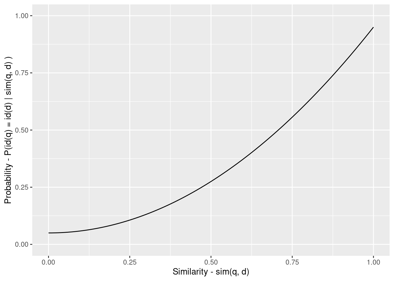
Figure 5.1: Example calibration from similarity to probability.
Figure 5.1 shows a hypothetical calibration from similarity to probability. Note that this is smooth and nonlinear and estimated from the oracle data.
6 Subpopulation calibration
The probability value of the calibration at any specific value of similarity is the expected probability where the expectation is effectively over the record pairs having that similarity value. Even if those record pairs have distinct, different probabilities the estimation of the calibration curve will summarise them to a single probability value.
This raises the possibility that the record pairs could be divided into subpopulations such that each subpopulation has a distinct calibration curve. If those subpopulations can be defined in terms of features derivable from the record pairs this indicates that there is information that could be exploited to make the similarity function more discriminating.
This predictive information could be used to estimate a new more discriminating similarity function. However, it may be more transparent to leave the similarity function (say, edit distance) unaltered and estimate separate calibration functions for each subpopulation. These are used to transform the similarities to probabilities and the populations can then be pooled.
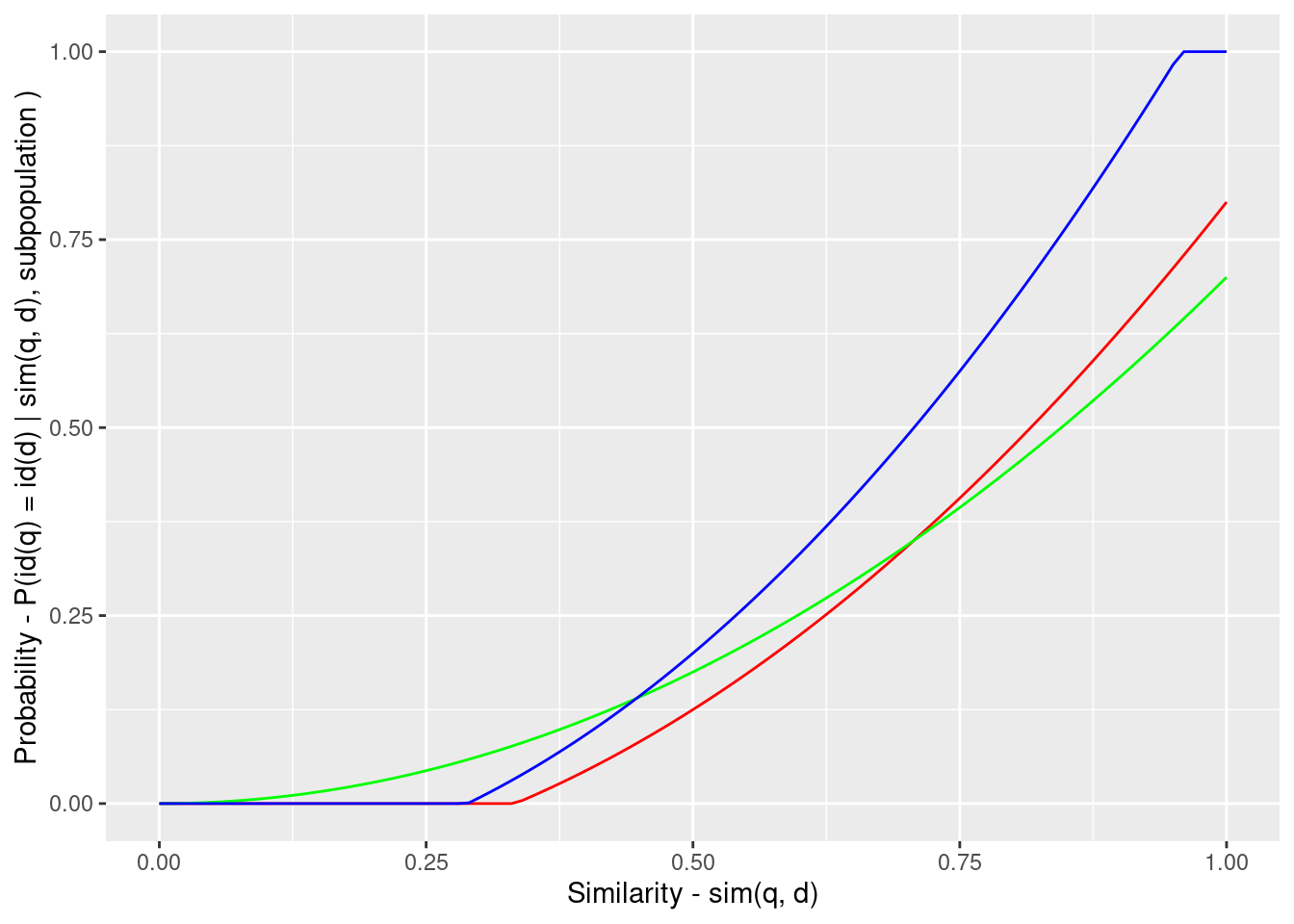
Figure 6.1: Example calibration of multiple subpopulations, each with a different calibration curve.
Figure 6.1 shows a hypothetical calibration from similarity to probability where the calibration relationship differs between subpopulations of record pairs. By applying the appropriate calibration function to each similarity value each similarity is transformed to a “true” probability so that the values can be pooled without concern for the subpopulation. This composition of the calibration and similarity functions can be viewed as yielding a function from record pairs to probability that takes similarity and subpopulation into account.
7 Construal as an interaction
The subpopulation-specific calibration can be interpreted as a statistical interaction. That is, the effect of similarity on probability depends on the value of subpopulation. Subpopulation membership is a discrete variable. However, interactions can also involve continuous variables. If there are any continuous variables derivable from the record pairs that have a strong impact on the similarity to probability calibration then it will be advantageous to exploit those variables in interactions with similarity.
8 Frequency-aware similarity
Consider the case where the codomains of the query and dictionary observation functions are the single attribute family_name. Person names have very skewed distributions, a small number of names (e.g. “Smith”) are relatively common, while most names (e.g. “Schwarzenegger”) are relatively rare. If the query and dictionary records are both “Smith” and the similarity function is exact equality the probability of identity will be quite low because there are multiple “Smith” dictionary records and only at most one has the same identity as the query record. Thus, the frequency of the value in the dictionary has a very strong effect on the probability corresponding to the level of similarity (exact equality). This is not a new observation (Lange & Naumann (2011)). The novel point here is that frequency can be exploited by using it in a statistical interaction with similarity.
The prior paragraph only covered the case where the similarity function is exact equality. How do we deal with the more usual case of a similarity function (e.g. edit distance) that returns a range of intermediate similarity values. This requires a digression into the interpretation of the probability \(P(id(q) = id(d) \mid q, d)\). The conditionality on \(q\) and \(d\) is equivalent to the fallible claim that \(q\) and \(d\) are observations of the same entity. Thus, \(P(id(q) = id(d) \mid q, d)\) can be read as, “Given the claim that \(q\) and \(d\) are observations of the same entity, what is the probability that claim is correct?” or “What is the probability that \(q\) and \(d\) are a true match?”
The probability \(P(id(q) = id(d) \mid sim(q, d) )\) treats all record pairs having the same similarity as identical and having an identical probability of being a true match. When directly using a similarity measure it is assumed that the probability of being a true match increases monotonically with the similarity (although this is not guaranteed and nonmonotonicity is known to occur). Assuming monotonicity and given \(q\) and \(d_i\) with similarity \(sim(q, d_i)\) - if we accept \(q\) and \(d_i\) as matching on the basis of that similarity then that implies we should also accept any \(d_j\) with \(sim(q, d_j) \ge sim(q, d_i)\) as a match. So the relevant frequency for frequency-aware similarity given a query record \(q\) and dictionary record \(d_i\) is the sum of the frequencies of all dictionary records \(d_j\) with similarity \(sim(q, d_j) \ge sim(q, d_i)\).
9 Curried similarity functions
We don’t know whether this is helpful, but it is at least mildly interesting that this approach can be viewed as creating curried similarity functions. We are only interested in one query record \(q\) at a time, although each query is run over every dictionary record \(d\) in \(D\). The frequency-aware calibration can be viewed as creating a modified similarity function \(sim_q(d)\) that is specific to the query \(q\), where the modification encodes the information in the relationship between \(q\) and all the \(d\) in \(D\).
10 Logistic regression
The standard statistical approach for modelling probabilities is logistic regression. Treating entity resolution as a statistical modelling problem allows the introduction of extra predictive variables as needed and gives access to the range of statistical practices and insights.
We intend to model frequency-aware similarity as a smooth interaction of frequency and similarity. This can be done with a generalised additive model, which is a type of generalised linear model, of which logistic regression is a special case.
The discussion in earlier sections has been in terms of observations having a single attribute. Treating entity resolution as a regression problem allows for straight-forward generalisation by adding multiple attributes as predictors.
References
R version 4.0.3 (2020-10-10)
Platform: x86_64-pc-linux-gnu (64-bit)
Running under: Ubuntu 20.10

Matrix products: default
BLAS:   /usr/lib/x86_64-linux-gnu/blas/libblas.so.3.9.0
LAPACK: /usr/lib/x86_64-linux-gnu/lapack/liblapack.so.3.9.0

locale:
 [1] LC_CTYPE=en_AU.UTF-8       LC_NUMERIC=C
 [3] LC_TIME=en_AU.UTF-8        LC_COLLATE=en_AU.UTF-8
 [5] LC_MONETARY=en_AU.UTF-8    LC_MESSAGES=en_AU.UTF-8
 [7] LC_PAPER=en_AU.UTF-8       LC_NAME=C
 [9] LC_ADDRESS=C               LC_TELEPHONE=C
[11] LC_MEASUREMENT=en_AU.UTF-8 LC_IDENTIFICATION=C

attached base packages:
[1] stats     graphics  grDevices datasets  utils     methods   base

other attached packages:
[1] ggplot2_3.3.3   magrittr_2.0.1  workflowr_1.6.2

loaded via a namespace (and not attached):
 [1] Rcpp_1.0.5       highr_0.8        pillar_1.4.7     compiler_4.0.3
 [5] later_1.1.0.1    git2r_0.27.1     tools_4.0.3      digest_0.6.27
 [9] evaluate_0.14    lifecycle_0.2.0  tibble_3.0.4     gtable_0.3.0
[13] pkgconfig_2.0.3  rlang_0.4.10     rstudioapi_0.13  yaml_2.2.1
[17] xfun_0.20        withr_2.3.0      stringr_1.4.0    dplyr_1.0.2
[21] knitr_1.30       generics_0.1.0   fs_1.5.0         vctrs_0.3.6
[25] tidyselect_1.1.0 rprojroot_2.0.2  grid_4.0.3       glue_1.4.2
[29] R6_2.5.0         rmarkdown_2.6    bookdown_0.21    farver_2.0.3
[33] purrr_0.3.4      whisker_0.4      scales_1.1.1     promises_1.1.1
[37] ellipsis_0.3.1   htmltools_0.5.0  colorspace_2.0-0 renv_0.12.4
[41] httpuv_1.5.4     labeling_0.4.2   stringi_1.5.3    munsell_0.5.0
[45] crayon_1.3.4