limma_analysis

Data Import

Set up DGElist object for downstream analysis and add sample-specific information and gene annotations.

# List count files from working directory
files <- list.files("./data/counts/", pattern = "_sorted\\.reverse_counts$")

# edgeR has a function readDGE for combining separate count files into one matrix of counts in one step
counts <- readDGE(files, path = "./data/counts/", columns = c(1,2), header = FALSE)

# Remove meta tags as library size includes counts from the meta tags
MetaTags <- grep("^__", rownames(counts))
counts <- counts[-MetaTags, ]

# Update library size to reflect mapped reads
counts$samples$lib.size <- colSums(counts$counts)

# Obtain sample names from file names
sample <- strsplit2(files, "_")[,1:3]
sample_names <- apply(sample, 1, function(row) paste(row, collapse = "_"))
counts$samples$mouse <- sample[,2]
counts$samples$pdx <- sample[,1]
replicates <- rep(c(1,1,1,2,2,2,3,3,3), times = 8)
counts$samples$replicates <- replicates
sample_name <- paste(counts$samples$pdx, counts$samples$replicates, sep = "_")
counts$samples$sample <- sample_name

# Add sample-level information related to experimental design (and possible confounding factors) to the count matrix
counts$samples$lane <- as.factor(strsplit2(files, "_")[,6])
counts$samples$pdx <- as.factor(sample[,1])

# Import information for each gene
geneid <- rownames(counts)
ensembl_ids <- sub("\\..*", "", geneid)
genes <- select(Homo.sapiens, keys=ensembl_ids, columns=c("SYMBOL", "TXCHROM", "ENTREZID"), 
                keytype="ENSEMBL")
genes <- genes[!duplicated(genes$ENSEMBL),]
counts$genes <- genes

# Remove genes without ENTREZ IDs
keep <- !is.na(counts$genes$ENTREZID) & !is.null(counts$genes$ENTREZID)
counts <- counts[keep, ]

The MDS plots below show that there is no batch effect from sequencing lane, so technical replicates run across the three lanes were summed together.

# Make MDS plots to assess technical replicate 
lcpm <- cpm(counts, log=TRUE)
col.pdx <- counts$samples$pdx
levels(col.pdx) <-  brewer.pal(nlevels(col.pdx), "Set1")
col.pdx <- as.character(col.pdx)
col.lane <- counts$samples$lane
levels(col.lane) <-  brewer.pal(nlevels(col.lane), "Set2")
col.lane <- as.character(col.lane)
plotMDS(lcpm, labels=counts$samples$sample, col=col.pdx)
title(main="A. Sample groups")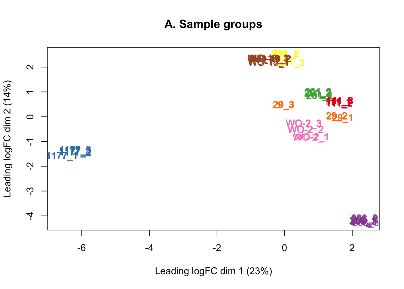

plotMDS(lcpm, labels=counts$samples$lane, col=col.lane)
title(main="B. Sequencing lanes")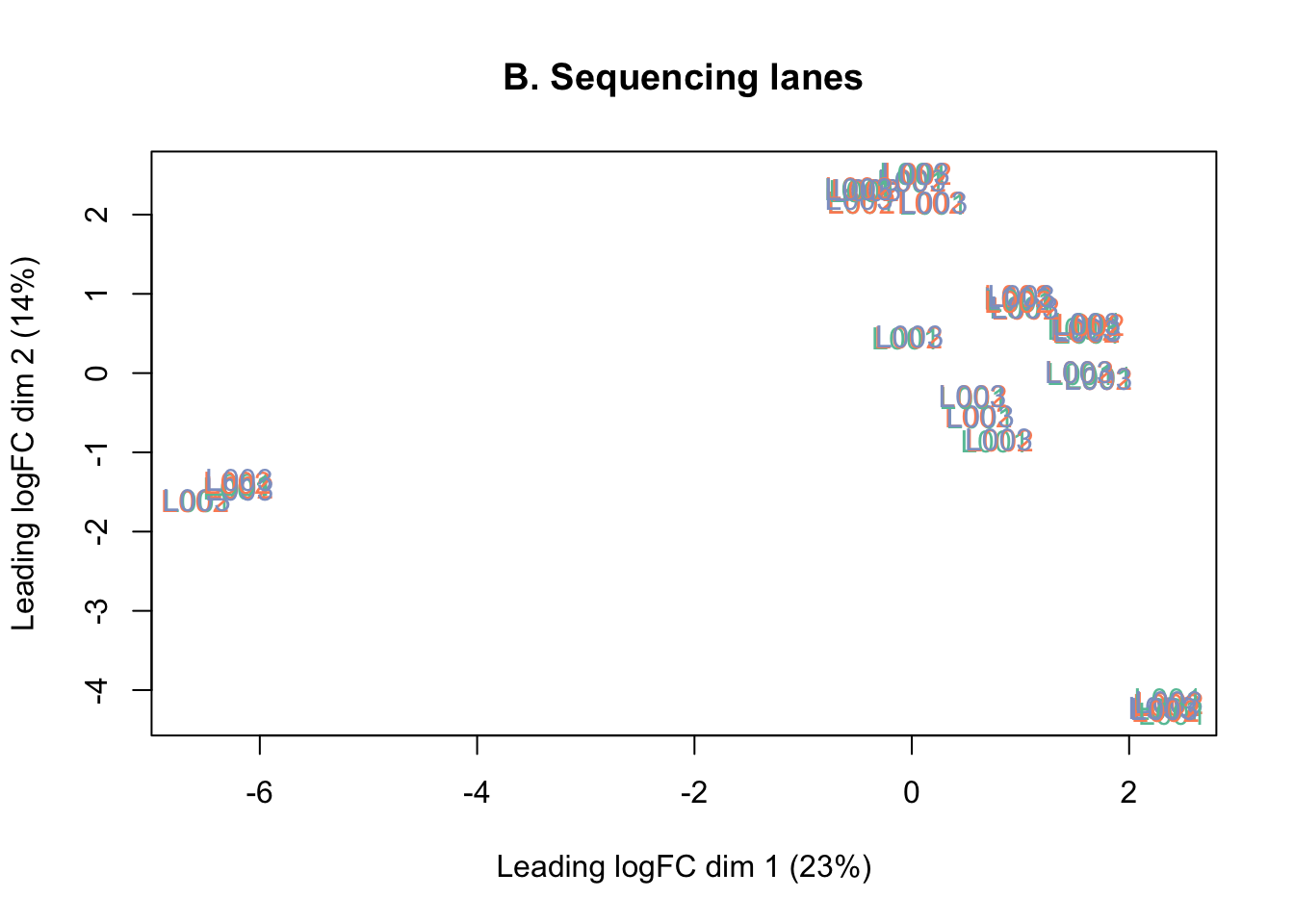

# Sum counts from technical replicates
samplenames <- counts$samples$sample
counts <- sumTechReps(counts, ID=samplenames)

# Add additional sample level information
elements <- c("response", "poor_response", "response", "poor_response", "response", "poor_response")
repeated_elements <- rep(elements, times = c(9,3,3,3,3,3))
group <- list(elements = repeated_elements)
counts$samples$group <- group$elements
elements <- c("1", "2")
repeated_elements <- rep(elements, times = c(18, 6))
site <- list(elements = repeated_elements)
counts$samples$site <- site$elements
elements <- c("HGSOC", "OCS","HGSOC")
repeated_elements <- rep(elements, times = c(3,3,18))
pathology <- list(elements = repeated_elements)
counts$samples$pathology <- pathology$elements
elements <- c("ovarian_tumour", "omental_tumour", "biopsy", "ovarian_tumour", "omental_tumour", "ovarian_tumour", "omental_tumour")
repeated_elements <- rep(elements, times = c(6,3,3,3,3,3,3))
specimen <- list(elements = repeated_elements)
counts$samples$specimen <- specimen$elements
elements <- c("refractory", "sensitive", "refractory", "resistant", "sensitive")
repeated_elements <- rep(elements, times = c(9,3,6,3,3))
platinum <- list(elements = repeated_elements)
counts$samples$platinum <- platinum$elements
replicates <- rep(1:3, times = 8)
counts$samples$replicates <- replicates
sample <- paste(counts$samples$pdx, counts$samples$replicates, sep = "_")
counts$samples$sample <- sample

# Generate library statistics
cpm <- cpm(counts)
lcpm <- cpm(counts, log=TRUE)
L <- mean(counts$samples$lib.size) * 1e-6
M <- median(counts$samples$lib.size) * 1e-6

Quality Control

Genes with no or low counts are unlikely to be biologically important, they provide little evidence for differential expression, and interfere with statistical approximations, so they were filtered out before performing the analysis. Genes with low or no counts (counts per million reads that corresponded to less than ~10 reads in any 9 samples (smallest group size)) were filtered out of the analysis, based on the recommendations in the edgeR documentation.

# Filter out genes with low expression
keep.exprs <- filterByExpr(counts, group=counts$samples$group)
table(keep.exprs)

keep.exprs
FALSE  TRUE 
18144 18314 

counts_filtered <- counts[keep.exprs,, keep.lib.sizes=FALSE]
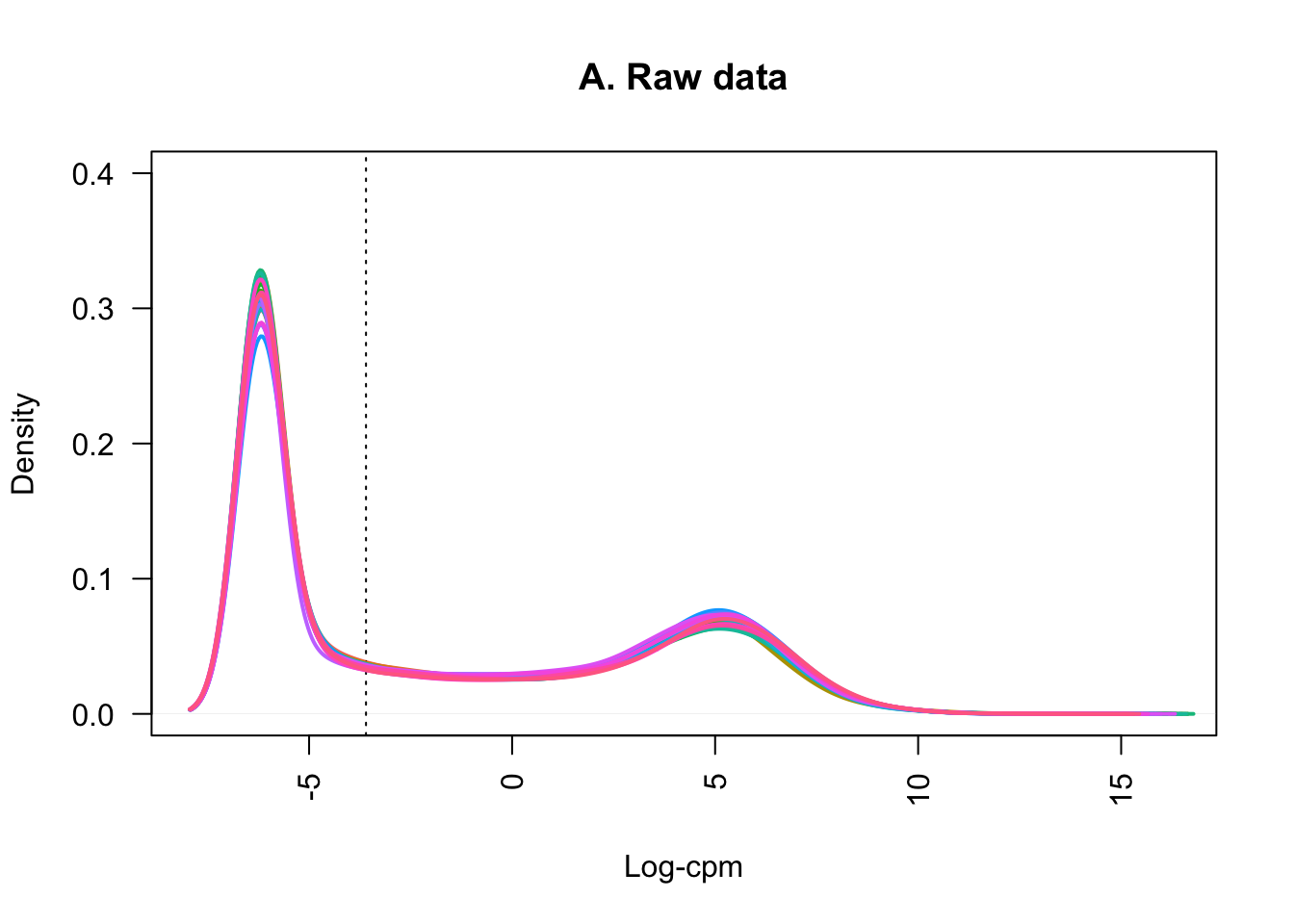
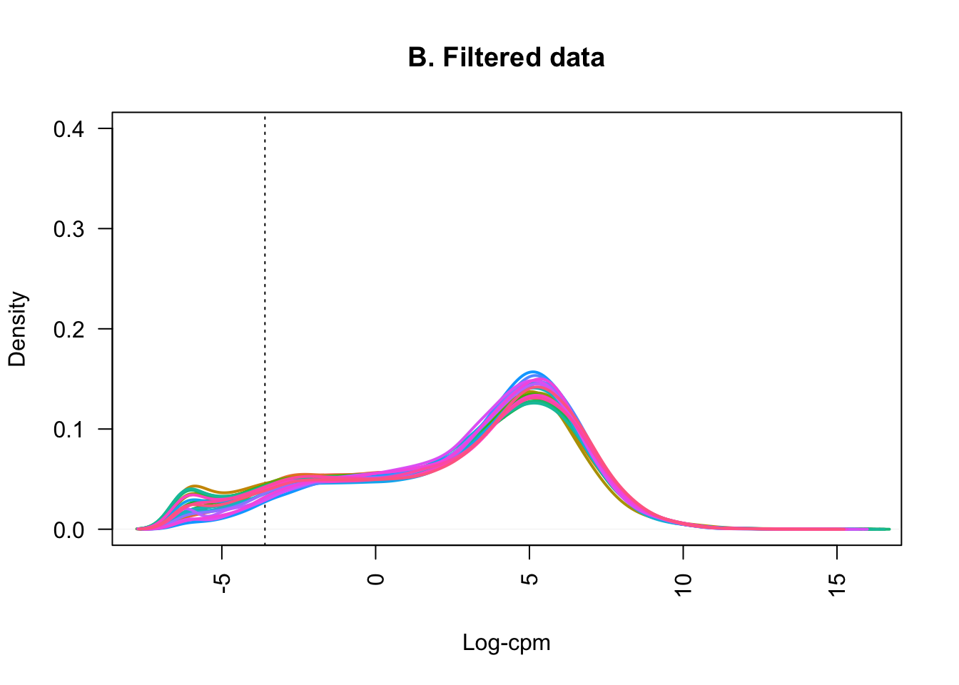
samplenames <- colnames(counts_filtered)

Plotting the distribution of log-CPM values (below) showed that before filtering (A) many genes in each sample had low or no expression, with negative log-CPM values. These genes were removed from the analysis after filtering (B).

# Make density plots for counts before and after filtering out genes with low expression
par(mfrow = c(1,1))
lcpmz <- lcpm
lcpm.cutoff <- log2(10/M + 2/L)
nsamples <- ncol(counts)
col <- scales::hue_pal()(nsamples)
plot(density(lcpm[,1]), col=col[1], lwd=2, ylim=c(0,0.4), las=2, main="", xlab="")
  title(main="A. Raw data", xlab="Log-cpm")
abline(v=lcpm.cutoff, lty=3)
for (i in 2:nsamples){
  den <- density(lcpm[,i])
  lines(den$x, den$y, col=col[i], lwd=2)
}

lcpm2 <- cpm(counts_filtered, log=TRUE)
plot(density(lcpm2[,1]), col=col[1], lwd=2, ylim=c(0,0.4), las=2, main="", xlab="")
title(main="B. Filtered data", xlab="Log-cpm")
abline(v=lcpm.cutoff, lty=3)
for (i in 2:nsamples){
  den <- density(lcpm2[,i])
  lines(den$x, den$y, col=col[i], lwd=2)
}

TMM normalisation was applied to account for any highly expressed genes monopolising the sequencing and to account for the underlying differences in the distributions of expressed genes between samples.

# Apply TMM normalisation
norm_counts <- calcNormFactors(counts_filtered, method = "TMM")

Effective library sizes varied from around 50 million reads to more than 250 million reads, with the median just under 150 million reads (A). The range and distribution of expression values looked fairly uniform between samples, and TMM normalisation further improved this.

dat <- data.frame(lib = norm_counts$samples$lib.size,
                  status = norm_counts$samples$group,
                  sample = colnames(norm_counts))
p1 <- ggplot(dat, aes(x = sample, y = lib, fill = status)) +
  geom_bar(stat = "identity") +
  theme(axis.text.x = element_text(angle = 45, hjust = 1)) +
  labs(x = "Sample", y = "Library size",
       fill = "CHK1i", title = "A. Library size after filtering") +
  geom_hline(yintercept = median(dat$lib), linetype = "dashed") +
  scale_x_discrete(limits = dat$sample)

dat <- reshape2::melt(cpm(norm_counts, normalized.lib.sizes = FALSE, log = TRUE),
                      value.name = "cpm")
dat$status <- rep(norm_counts$samples$group, each = nrow(norm_counts))
colnames(dat)[2] <- "sample"
p2 <- ggplot(dat, aes(x = sample, y = cpm, fill = status)) +
  geom_boxplot(show.legend = FALSE, outlier.size = 0.75) +
  theme(axis.text.x = element_text(angle = 45, hjust = 1, size = 7)) +
  labs(x = "Sample", y = "Log-CPM",
       fill = "CHK1i treatment", title = "B. Expression values after filtering") +
  geom_hline(yintercept = median(dat$lib), linetype = "dashed")

dat <- reshape2::melt(cpm(norm_counts, normalized.lib.sizes = TRUE, log = TRUE),
                      value.name = "cpm")

dat$status <- rep(norm_counts$samples$group, each = nrow(norm_counts))
colnames(dat)[2] <- "sample"
p3 <- ggplot(dat, aes(x = sample, y = cpm, fill = status)) +
  geom_boxplot(show.legend = FALSE, outlier.size = 0.75) +
  theme(axis.text.x = element_text(angle = 45, hjust = 1, size = 7)) +
  labs(x = "Sample", y = "Log-CPM",
       fill = "CHK1i treatment", title = "C. Expression values after normalisation") +
  geom_hline(yintercept = median(dat$lib), linetype = "dashed")

p1 / (p2 + p3) + plot_layout(guides = "collect")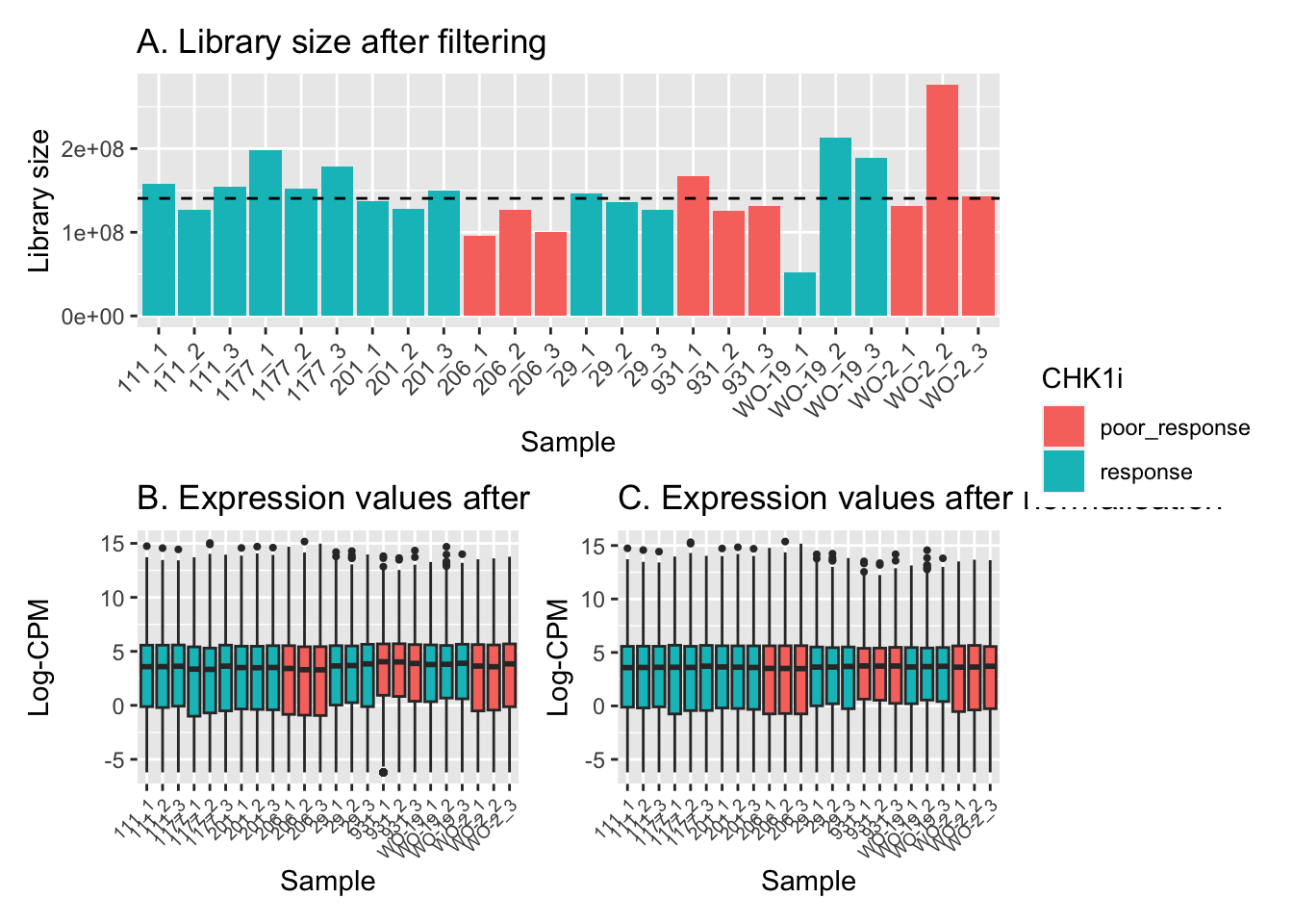

Multi-dimensional scaling (MDS) plots show the largest sources of variation in the data. They are a good way of identifying structure in the data and exploring relationships between samples. The following plots examine the first dimensions coloured for known features of the data. The samples do not cluster in any of the first dimensions based on their CHK1i responder status, suggesting that this is not the largest source of variation in the data. Sample 1177 is an outlier in the first dimension, which is confounded with it being the only OCS sample. Sample 206 also appears like it may be an outlier in dimension 2, this may correspond to it being the only biopsy specimen. The remaining samples cluster reasonably closely together, except for WO-2, which is a bit closer to 206 in the first and second dimensions, which may reflect that these are the only two platinum sensitive pdx models. Overall, the large amount of variation in the first dimension suggests that there might be tumour specific differences in expression driving the variation.

dims <- list(c(1,2), c(1,3), c(2,3), c(3,4))
vars <- c("group", "pdx", "site", "pathology", "specimen", "platinum")
patches <- vector("list", length(vars))

for(i in 1:length(vars)){
  p <- vector("list", length(dims))
  
  for(j in 1:length(dims)){
    mds <- plotMDS(cpm(norm_counts, log = TRUE), top = 1000, gene.selection="common", 
                   plot = FALSE, dim.plot = dims[[j]])
    dat <- tibble::tibble(x = mds$x, y = mds$y,
                          sample = norm_counts$samples$sample,
                          variable = pull(norm_counts$samples, vars[i]))
    
    p[[j]] <- ggplot(dat, aes(x = x, y = y, colour = variable)) +
      geom_text(aes(label = sample), size = 2.5) +
      labs(x = glue::glue("Leading logFC dim {dims[[j]][1]}"), 
           y = glue::glue("Leading logFC dim {dims[[j]][2]}"),
           colour = vars[i])
  }
  
  patches[[i]] <- wrap_elements(wrap_plots(p, ncol = 2, guides = "collect") +
    plot_annotation(title = glue::glue("Coloured by: {vars[i]}")) &
    theme(legend.position = "bottom"))
  
}

patches

[[1]]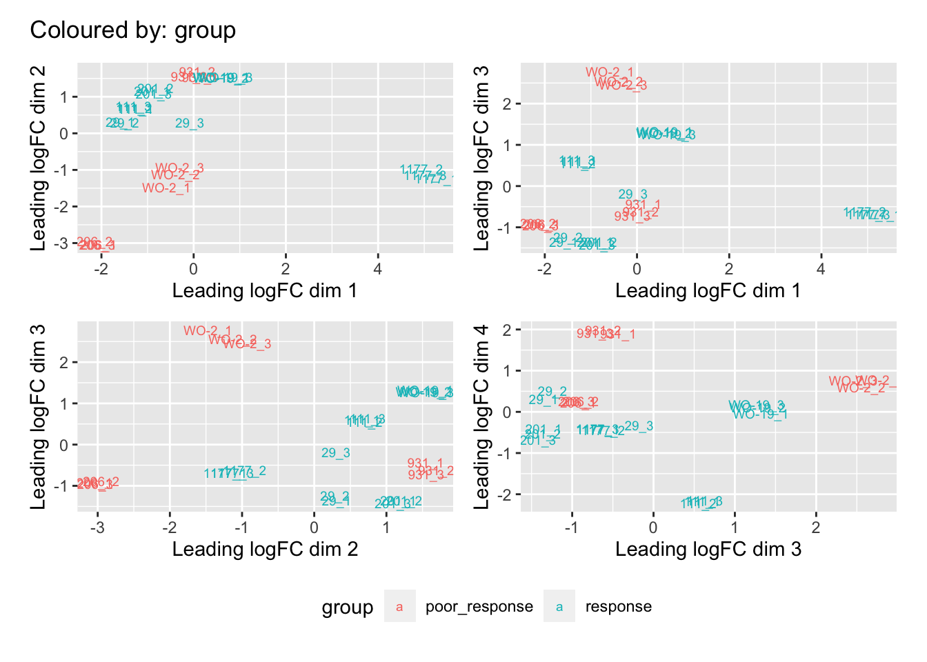

[[2]]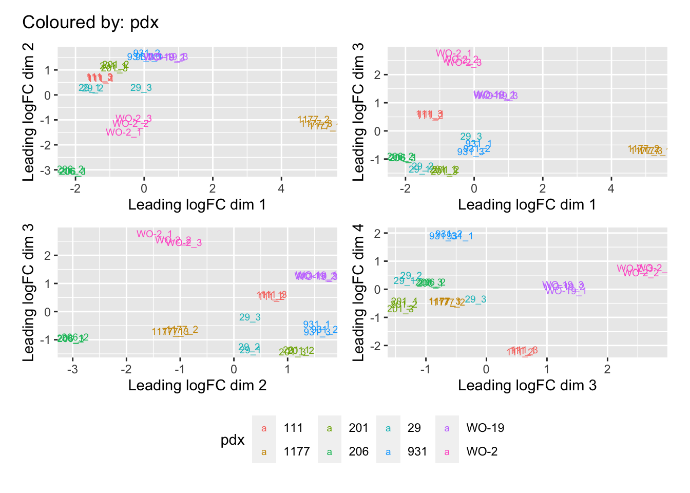

[[3]]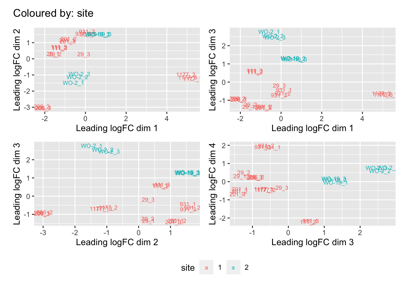

[[4]]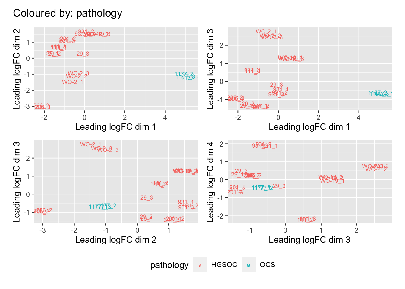

[[5]]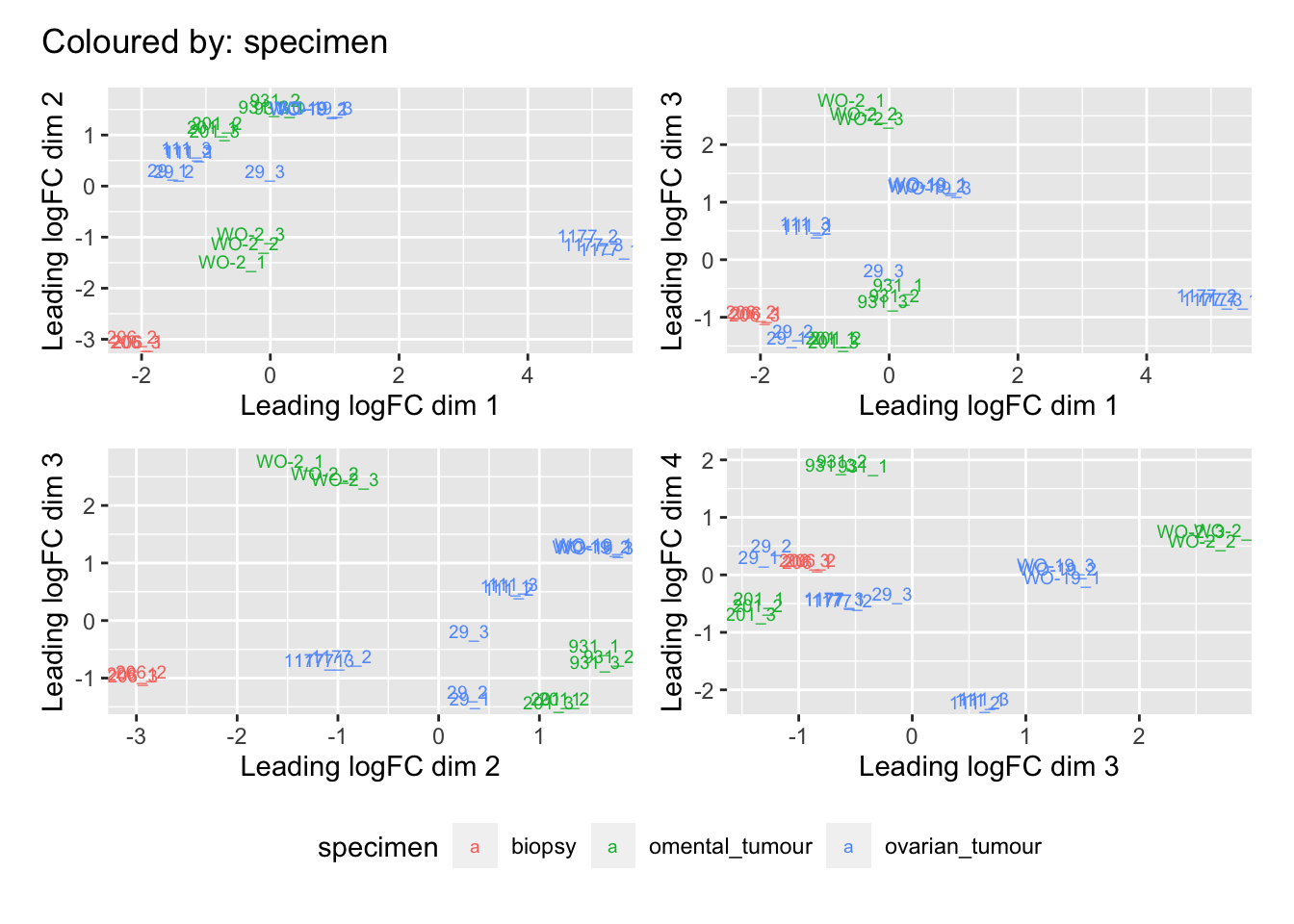

[[6]]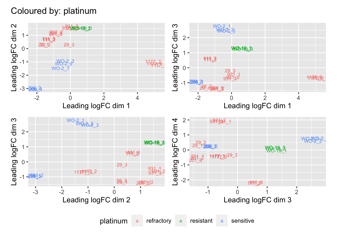

# Create MDS plot for supplementary figure

dims <- list(c(1, 2), c(1, 3), c(2, 3), c(3, 4))

# Create a list to store the MDS plots
mds_plots <- list()

for (i in 1:length(dims)) {
  mds <- plotMDS(cpm(norm_counts, log = TRUE), top = 1000, gene.selection = "common", 
                 plot = FALSE, dim.plot = dims[[i]])
  
  dat <- tibble::tibble(x = mds$x, y = mds$y,
                        pdx = pull(norm_counts$samples, "pdx"),
                        group = pull(norm_counts$samples, "group"),
                        pathology = pull(norm_counts$samples, "pathology"))
  
  p <- ggplot(dat, aes(x = x, y = y)) +
    geom_point(aes(color = pdx, shape = group, fill = pathology), size = 3) +
    scale_shape_manual(values = c("response" = 16, "poor_response" = 17)) +
    labs(x = glue::glue("Leading logFC dim {dims[[i]][1]}"), 
         y = glue::glue("Leading logFC dim {dims[[i]][2]}")) +
    theme(legend.position = "none")  # Remove individual legends
  
  # Add a circle around points with pathology "OCS" using ggforce
  p <- p + geom_circle(data = filter(dat, pathology == "OCS"), 
                        aes(x0 = x, y0 = y, r = 0.2), 
                        color = "grey", fill = NA, size = 1)
  
  mds_plots[[i]] <- p
}

# Combine the MDS plots into a single plot
mds_arranged <- plot_grid(
  plot_grid(mds_plots[[1]], mds_plots[[2]], ncol = 2) + theme(legend.position = "none"),
  plot_grid(mds_plots[[3]], mds_plots[[4]], ncol = 2) + theme(legend.position = "none"),
  nrow = 2
)
# Display the arranged MDS plots
print(mds_arranged)

Differential expression analysis

In the following analysis, a test is set up to compare responders with non-responders, excluding outlier sample 1177. A means model was fitted where the model parameters represent the means of each pdx model, and responsive models were compared to non-responsive models by testing the difference between the parameter estimates in each group.

# Set up design matrix with parameter for each pdx model
pdx <- as.factor(norm_counts$samples$pdx)
design1 <- model.matrix(~0 + pdx)
colnames(design1) <- gsub("group", "", colnames(design1))
new_names <- c("pdxWO_19", "pdxWO_2")
old_names <- c("pdxWO-19", "pdxWO-2")
for (i in 1:length(old_names)) {
  colnames(design1)[colnames(design1) == old_names[i]] <- new_names[i]
}
rownames(design1) <- samplenames

# Set up contrast to test responsive versus non-responsive models
contrast <- makeContrasts(
  resp.v.nonresp = (pdx29+pdx111+pdx201+pdxWO_19)/4-(pdx206+pdx931+pdxWO_2)/3,
  levels=colnames(design1))

Apply linear modelling using the limma function, which uses the log-CPM values which are assumed to be normally distributed, with precision-weights calculated by the voom function for the mean-variance relationship. Number of significant genes listed below in table 1.

# Apply voom function to the normalised counts
par(mfrow=c(1,2))
v <- voom(norm_counts, design1, plot=TRUE)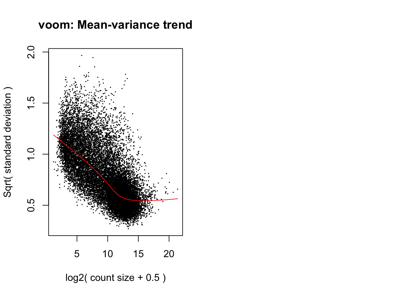

# Fit linear model and apply contrast for test
vfit <- lmFit(v, design1)
vfit.cont <- contrasts.fit(vfit, contrasts=contrast)
efit <- eBayes(vfit.cont)
plotSA(efit, main="Final model: Mean-variance trend")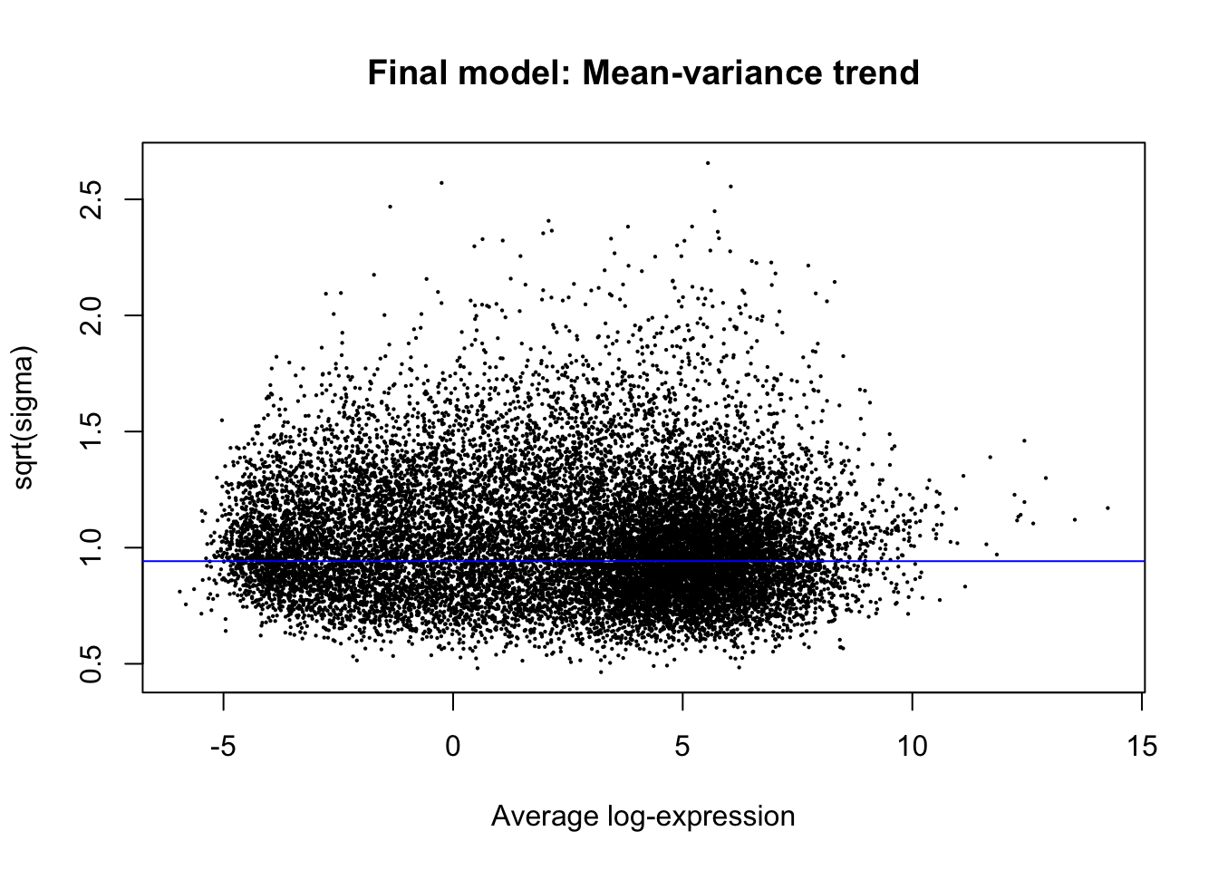

# Find number of differentially expressed genes
kable_styling(kable(summary(decideTests(efit)), caption="Table 1: Number of differentially expressed genes"))

Since the number of differentially expressed genes was very high, the treat method was applied to set a fold change cutoff of 0.5, which reduced the number of significant genes to a more manageable number. Table 2 shows the number of significantly differentially expressed genes after applying the fold change cut off and running each of the tests. Table 3 shows the top 20 DE genes for responder vs poor responder test.

# Apply log fold change cutoff to find significant genes
tfit <- treat(vfit.cont, lfc=0.5)

# Make table with number of DEGs for each test
dt <- decideTests(tfit)
kable_styling(kable(summary(dt, caption="Table 2: Number of differentially expressed genes from treat method")))

# Make table with top DEGs for each test
top_treat_resp.v.nonresp <- data.frame(topTreat(tfit, n=20, sort.by = "P"))
kable_styling(kable(top_treat_resp.v.nonresp[,c(3,5,6,9)], caption="Table 3: DE genes in responsive pdx versus poor responders", digits = 20))

To look at the levels of gene expression in individual samples the GlMDPlot function was used. This creates a two-panel interactive MD plot in an html. The left plot shows the log-fold-change vs average expression with up regulated genes coloured red and down regulated genes coloured blue. The right plot shows the expression levels of a particular gene in each sample, grouped by pdx model. Hovering over points on left plot will plot expression level for the corresponding gene, clicking on points will fix the expression plot to gene. Clicking on a row in the table has the same effect as clicking on the corresponding gene in the plot. The values in the table correspond to the test of responders versus non-responders excluding outlier pdx 1177 samples.

lcpm <- cpm(norm_counts, log=TRUE)
glMDPlot(tfit, coef = 1, counts = lcpm, status=dt, main="MD plot: Responders versus poor responders", groups=pdx)

Click here to see interactive MD plot

Investigating the top genes shows that many of the genes called as differentially expressed are actually being driven by just one PDX model, and not reflective of the difference between responders and poor responders.

Below is a basic heatmap made using the expression of the top 200 genes. As expected from the PCA plots and visualisations, pdx 206 is behaving very differently to the other samples for a subset of genes. Also sample 931 clusters with the responders rather than the non-responders.

# Specify color palette from RColorBrewer
my_palette <- colorRampPalette(brewer.pal(9, "RdBu"))(100)
group_colours <- c("response" = brewer.pal(8, "Set2")[1],  # Green
                   "poor_response" = brewer.pal(8, "Set2")[4])  # Pink

# Create a legend
legend_labels <- unique(unlist(group))
legend_colours <- group_colours[legend_labels]

legend_text <- c("Responders", "Poor responders")

# Make heatmap using heatmap.2
dge <- data.frame(topTreat(tfit, n=Inf, sort.by = "P"))
lcpm2 <- lcpm[, -c(4:6)]
responsive.v.non <- dge$ENSEMBL[1:200]
i <- which(norm_counts$genes$ENSEMBL %in% responsive.v.non)
heatmap.2(lcpm2[i,], scale="row",
   labRow=norm_counts$genes$SYMBOL[i], labCol=colnames(lcpm2), 
   col=my_palette, trace="none", density.info="none", 
   margin=c(8,6), lhei=c(2,10), dendrogram="column", key.title = "Expression Levels",
   ColSideColors = group_colours[unlist(group)[4:24]],
   cexCol = 1.8)

# Add the legend to the plot
legend("left", legend = legend_text, fill = legend_colours, title = "Sample Groups")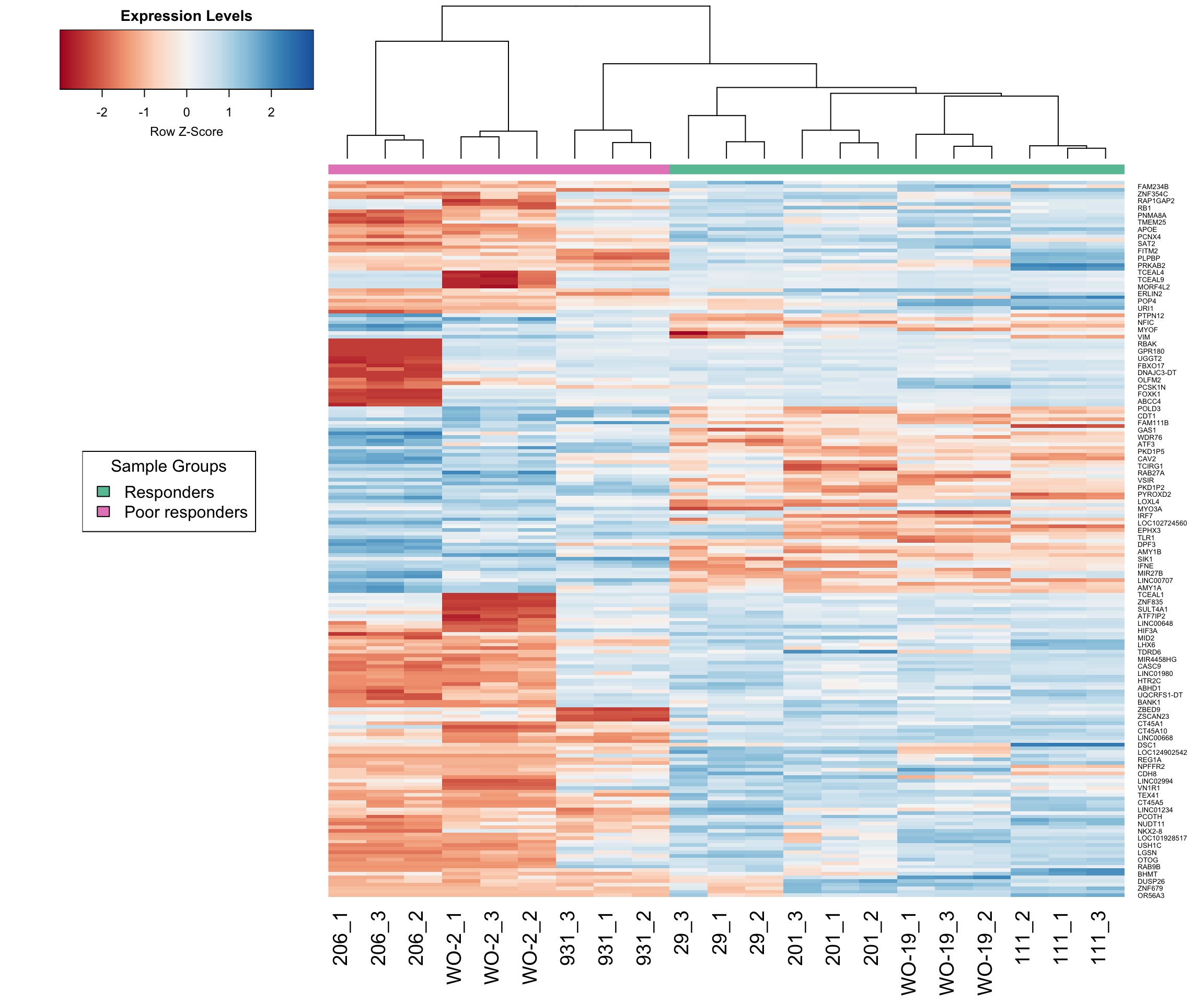

sessionInfo()

R version 4.2.2 (2022-10-31)
Platform: aarch64-apple-darwin20 (64-bit)
Running under: macOS Monterey 12.5.1

Matrix products: default
BLAS:   /Library/Frameworks/R.framework/Versions/4.2-arm64/Resources/lib/libRblas.0.dylib
LAPACK: /Library/Frameworks/R.framework/Versions/4.2-arm64/Resources/lib/libRlapack.dylib

locale:
[1] en_US.UTF-8/en_US.UTF-8/en_US.UTF-8/C/en_US.UTF-8/en_US.UTF-8

attached base packages:
[1] stats4    stats     graphics  grDevices utils     datasets  methods  
[8] base     

other attached packages:
 [1] ggforce_0.4.1                          
 [2] cowplot_1.1.1                          
 [3] glue_1.6.2                             
 [4] Glimma_2.8.0                           
 [5] gplots_3.1.3                           
 [6] ggrepel_0.9.4                          
 [7] kableExtra_1.3.4                       
 [8] knitr_1.44                             
 [9] patchwork_1.1.3                        
[10] Homo.sapiens_1.3.1                     
[11] TxDb.Hsapiens.UCSC.hg19.knownGene_3.2.2
[12] org.Hs.eg.db_3.16.0                    
[13] GO.db_3.16.0                           
[14] OrganismDbi_1.40.0                     
[15] GenomicFeatures_1.50.4                 
[16] GenomicRanges_1.50.2                   
[17] GenomeInfoDb_1.34.9                    
[18] AnnotationDbi_1.60.2                   
[19] IRanges_2.32.0                         
[20] S4Vectors_0.36.2                       
[21] Biobase_2.58.0                         
[22] BiocGenerics_0.44.0                    
[23] RColorBrewer_1.1-3                     
[24] lubridate_1.9.3                        
[25] forcats_1.0.0                          
[26] stringr_1.5.0                          
[27] dplyr_1.1.3                            
[28] purrr_1.0.2                            
[29] readr_2.1.4                            
[30] tidyr_1.3.0                            
[31] tibble_3.2.1                           
[32] ggplot2_3.4.4                          
[33] tidyverse_2.0.0                        
[34] edgeR_3.40.2                           
[35] limma_3.54.2                           
[36] here_1.0.1                             
[37] workflowr_1.7.1                        

loaded via a namespace (and not attached):
  [1] BiocFileCache_2.6.1         systemfonts_1.0.5          
  [3] plyr_1.8.9                  BiocParallel_1.32.6        
  [5] digest_0.6.33               htmltools_0.5.6.1          
  [7] fansi_1.0.5                 magrittr_2.0.3             
  [9] memoise_2.0.1               tzdb_0.4.0                 
 [11] annotate_1.76.0             Biostrings_2.66.0          
 [13] matrixStats_1.0.0           svglite_2.1.2              
 [15] timechange_0.2.0            prettyunits_1.2.0          
 [17] colorspace_2.1-0            blob_1.2.4                 
 [19] rvest_1.0.3                 rappdirs_0.3.3             
 [21] xfun_0.40                   callr_3.7.3                
 [23] crayon_1.5.2                RCurl_1.98-1.12            
 [25] jsonlite_1.8.7              graph_1.76.0               
 [27] polyclip_1.10-6             gtable_0.3.4               
 [29] zlibbioc_1.44.0             XVector_0.38.0             
 [31] webshot_0.5.5               DelayedArray_0.24.0        
 [33] scales_1.2.1                DBI_1.1.3                  
 [35] Rcpp_1.0.11                 xtable_1.8-4               
 [37] viridisLite_0.4.2           progress_1.2.2             
 [39] bit_4.0.5                   htmlwidgets_1.6.2          
 [41] httr_1.4.7                  farver_2.1.1               
 [43] pkgconfig_2.0.3             XML_3.99-0.14              
 [45] sass_0.4.7                  dbplyr_2.4.0               
 [47] locfit_1.5-9.8              utf8_1.2.4                 
 [49] labeling_0.4.3              reshape2_1.4.4             
 [51] tidyselect_1.2.0            rlang_1.1.1                
 [53] later_1.3.1                 munsell_0.5.0              
 [55] tools_4.2.2                 cachem_1.0.8               
 [57] cli_3.6.1                   generics_0.1.3             
 [59] RSQLite_2.3.2               evaluate_0.22              
 [61] fastmap_1.1.1               yaml_2.3.7                 
 [63] processx_3.8.2              bit64_4.0.5                
 [65] fs_1.6.3                    caTools_1.18.2             
 [67] KEGGREST_1.38.0             RBGL_1.74.0                
 [69] whisker_0.4.1               xml2_1.3.5                 
 [71] biomaRt_2.54.1              compiler_4.2.2             
 [73] rstudioapi_0.15.0           filelock_1.0.2             
 [75] curl_5.1.0                  png_0.1-8                  
 [77] tweenr_2.0.2                geneplotter_1.76.0         
 [79] bslib_0.5.1                 stringi_1.7.12             
 [81] highr_0.10                  ps_1.7.5                   
 [83] lattice_0.22-5              Matrix_1.6-1.1             
 [85] vctrs_0.6.4                 pillar_1.9.0               
 [87] lifecycle_1.0.3             BiocManager_1.30.22        
 [89] jquerylib_0.1.4             bitops_1.0-7               
 [91] httpuv_1.6.12               rtracklayer_1.58.0         
 [93] R6_2.5.1                    BiocIO_1.8.0               
 [95] promises_1.2.1              KernSmooth_2.23-22         
 [97] codetools_0.2-19            MASS_7.3-60                
 [99] gtools_3.9.4                SummarizedExperiment_1.28.0
[101] DESeq2_1.38.3               rprojroot_2.0.3            
[103] rjson_0.2.21                withr_2.5.1                
[105] GenomicAlignments_1.34.1    Rsamtools_2.14.0           
[107] GenomeInfoDbData_1.2.9      parallel_4.2.2             
[109] hms_1.1.3                   grid_4.2.2                 
[111] rmarkdown_2.25              MatrixGenerics_1.10.0      
[113] git2r_0.32.0                getPass_0.2-2              
[115] restfulr_0.0.15            

Session information

sessionInfo()

R version 4.2.2 (2022-10-31)
Platform: aarch64-apple-darwin20 (64-bit)
Running under: macOS Monterey 12.5.1

Matrix products: default
BLAS:   /Library/Frameworks/R.framework/Versions/4.2-arm64/Resources/lib/libRblas.0.dylib
LAPACK: /Library/Frameworks/R.framework/Versions/4.2-arm64/Resources/lib/libRlapack.dylib

locale:
[1] en_US.UTF-8/en_US.UTF-8/en_US.UTF-8/C/en_US.UTF-8/en_US.UTF-8

attached base packages:
[1] stats4    stats     graphics  grDevices utils     datasets  methods  
[8] base     

other attached packages:
 [1] ggforce_0.4.1                          
 [2] cowplot_1.1.1                          
 [3] glue_1.6.2                             
 [4] Glimma_2.8.0                           
 [5] gplots_3.1.3                           
 [6] ggrepel_0.9.4                          
 [7] kableExtra_1.3.4                       
 [8] knitr_1.44                             
 [9] patchwork_1.1.3                        
[10] Homo.sapiens_1.3.1                     
[11] TxDb.Hsapiens.UCSC.hg19.knownGene_3.2.2
[12] org.Hs.eg.db_3.16.0                    
[13] GO.db_3.16.0                           
[14] OrganismDbi_1.40.0                     
[15] GenomicFeatures_1.50.4                 
[16] GenomicRanges_1.50.2                   
[17] GenomeInfoDb_1.34.9                    
[18] AnnotationDbi_1.60.2                   
[19] IRanges_2.32.0                         
[20] S4Vectors_0.36.2                       
[21] Biobase_2.58.0                         
[22] BiocGenerics_0.44.0                    
[23] RColorBrewer_1.1-3                     
[24] lubridate_1.9.3                        
[25] forcats_1.0.0                          
[26] stringr_1.5.0                          
[27] dplyr_1.1.3                            
[28] purrr_1.0.2                            
[29] readr_2.1.4                            
[30] tidyr_1.3.0                            
[31] tibble_3.2.1                           
[32] ggplot2_3.4.4                          
[33] tidyverse_2.0.0                        
[34] edgeR_3.40.2                           
[35] limma_3.54.2                           
[36] here_1.0.1                             
[37] workflowr_1.7.1                        

loaded via a namespace (and not attached):
  [1] BiocFileCache_2.6.1         systemfonts_1.0.5          
  [3] plyr_1.8.9                  BiocParallel_1.32.6        
  [5] digest_0.6.33               htmltools_0.5.6.1          
  [7] fansi_1.0.5                 magrittr_2.0.3             
  [9] memoise_2.0.1               tzdb_0.4.0                 
 [11] annotate_1.76.0             Biostrings_2.66.0          
 [13] matrixStats_1.0.0           svglite_2.1.2              
 [15] timechange_0.2.0            prettyunits_1.2.0          
 [17] colorspace_2.1-0            blob_1.2.4                 
 [19] rvest_1.0.3                 rappdirs_0.3.3             
 [21] xfun_0.40                   callr_3.7.3                
 [23] crayon_1.5.2                RCurl_1.98-1.12            
 [25] jsonlite_1.8.7              graph_1.76.0               
 [27] polyclip_1.10-6             gtable_0.3.4               
 [29] zlibbioc_1.44.0             XVector_0.38.0             
 [31] webshot_0.5.5               DelayedArray_0.24.0        
 [33] scales_1.2.1                DBI_1.1.3                  
 [35] Rcpp_1.0.11                 xtable_1.8-4               
 [37] viridisLite_0.4.2           progress_1.2.2             
 [39] bit_4.0.5                   htmlwidgets_1.6.2          
 [41] httr_1.4.7                  farver_2.1.1               
 [43] pkgconfig_2.0.3             XML_3.99-0.14              
 [45] sass_0.4.7                  dbplyr_2.4.0               
 [47] locfit_1.5-9.8              utf8_1.2.4                 
 [49] labeling_0.4.3              reshape2_1.4.4             
 [51] tidyselect_1.2.0            rlang_1.1.1                
 [53] later_1.3.1                 munsell_0.5.0              
 [55] tools_4.2.2                 cachem_1.0.8               
 [57] cli_3.6.1                   generics_0.1.3             
 [59] RSQLite_2.3.2               evaluate_0.22              
 [61] fastmap_1.1.1               yaml_2.3.7                 
 [63] processx_3.8.2              bit64_4.0.5                
 [65] fs_1.6.3                    caTools_1.18.2             
 [67] KEGGREST_1.38.0             RBGL_1.74.0                
 [69] whisker_0.4.1               xml2_1.3.5                 
 [71] biomaRt_2.54.1              compiler_4.2.2             
 [73] rstudioapi_0.15.0           filelock_1.0.2             
 [75] curl_5.1.0                  png_0.1-8                  
 [77] tweenr_2.0.2                geneplotter_1.76.0         
 [79] bslib_0.5.1                 stringi_1.7.12             
 [81] highr_0.10                  ps_1.7.5                   
 [83] lattice_0.22-5              Matrix_1.6-1.1             
 [85] vctrs_0.6.4                 pillar_1.9.0               
 [87] lifecycle_1.0.3             BiocManager_1.30.22        
 [89] jquerylib_0.1.4             bitops_1.0-7               
 [91] httpuv_1.6.12               rtracklayer_1.58.0         
 [93] R6_2.5.1                    BiocIO_1.8.0               
 [95] promises_1.2.1              KernSmooth_2.23-22         
 [97] codetools_0.2-19            MASS_7.3-60                
 [99] gtools_3.9.4                SummarizedExperiment_1.28.0
[101] DESeq2_1.38.3               rprojroot_2.0.3            
[103] rjson_0.2.21                withr_2.5.1                
[105] GenomicAlignments_1.34.1    Rsamtools_2.14.0           
[107] GenomeInfoDbData_1.2.9      parallel_4.2.2             
[109] hms_1.1.3                   grid_4.2.2                 
[111] rmarkdown_2.25              MatrixGenerics_1.10.0      
[113] git2r_0.32.0                getPass_0.2-2              
[115] restfulr_0.0.15