Analyze_PrediXcan_Results
sabrina-mi
2022-08-22
Last updated: 2022-08-22
Checks: 6 1
Knit directory: RatXcan_Training/
This reproducible R Markdown analysis was created with workflowr (version 1.6.2). The Checks tab describes the reproducibility checks that were applied when the results were created. The Past versions tab lists the development history.
The R Markdown is untracked by Git. To know which version of the R
Markdown file created these results, you’ll want to first commit it to
the Git repo. If you’re still working on the analysis, you can ignore
this warning. When you’re finished, you can run
wflow_publish to commit the R Markdown file and build the
HTML.
Great job! The global environment was empty. Objects defined in the global environment can affect the analysis in your R Markdown file in unknown ways. For reproduciblity it’s best to always run the code in an empty environment.
The command set.seed(20220711) was run prior to running
the code in the R Markdown file. Setting a seed ensures that any results
that rely on randomness, e.g. subsampling or permutations, are
reproducible.
Great job! Recording the operating system, R version, and package versions is critical for reproducibility.
Nice! There were no cached chunks for this analysis, so you can be confident that you successfully produced the results during this run.
Great job! Using relative paths to the files within your workflowr project makes it easier to run your code on other machines.
Great! You are using Git for version control. Tracking code development and connecting the code version to the results is critical for reproducibility.
The results in this page were generated with repository version 6e9507f. See the Past versions tab to see a history of the changes made to the R Markdown and HTML files.
Note that you need to be careful to ensure that all relevant files for
the analysis have been committed to Git prior to generating the results
(you can use wflow_publish or
wflow_git_commit). workflowr only checks the R Markdown
file, but you know if there are other scripts or data files that it
depends on. Below is the status of the Git repository when the results
were generated:
Ignored files:
    Ignored:    .Rhistory
    Ignored:    .Rproj.user/
    Ignored:    analysis/.Rhistory
    Ignored:    output/
    Ignored:    scripts/.Rhistory

Untracked files:
    Untracked:  .DS_Store
    Untracked:  .gitignore
    Untracked:  analysis/Analyze_PrediXcan_Results.Rmd
    Untracked:  analysis/figure/

Unstaged changes:
    Modified:   analysis/.DS_Store
    Modified:   analysis/EN_Prediction_Model.Rmd
    Modified:   analysis/Rat_PTRS.Rmd
    Modified:   analysis/Run_PrediXcan.Rmd
    Modified:   analysis/index.Rmd
Note that any generated files, e.g. HTML, png, CSS, etc., are not included in this status report because it is ok for generated content to have uncommitted changes.
There are no past versions. Publish this analysis with
wflow_publish() to start tracking its development.
Identify Significant Genes
library(readr)
library(tidyverse)
── Attaching packages ─────────────────────────────────────── tidyverse 1.3.0 ──✔ ggplot2 3.3.6 ✔ dplyr 1.0.2
✔ tibble 3.0.4 ✔ stringr 1.4.0
✔ tidyr 1.1.2 ✔ forcats 0.5.0
✔ purrr 0.3.4 ── Conflicts ────────────────────────────────────────── tidyverse_conflicts() ──
✖ dplyr::filter() masks stats::filter()
✖ dplyr::lag() masks stats::lag()tis="Ac"
"%&%" = function(a,b) paste(a,b,sep="")
dir="/Users/sabrinami/Library/CloudStorage/Box-Box/imlab-data/data-Github/Rat_Genomics_Paper_Pipeline/"Read in association results for each phenotype, and combine in one dataframe.
library(stringr)
filelist <- list.files(dir %&% "Results/PrediXcan/metabolic_traits", pattern = "Ac__association_", full.names = TRUE)
full_df <- data.frame()

for(file in filelist) {
  assoc_file <- read_tsv(file, col_names = TRUE)
  # extract phenotype from regex matching in file name
  pheno_id <- str_match(file, "association_(.*?).txt")[,2]
  tempo <- cbind(assoc_file, metabolic_trait=pheno_id) %>% select(-c(status))
  full_df <- rbind(full_df, tempo)
}
── Column specification ────────────────────────────────────────────────────────
cols(
  gene = col_character(),
  effect = col_double(),
  se = col_double(),
  zscore = col_double(),
  pvalue = col_double(),
  n_samples = col_double(),
  status = col_logical()
)


── Column specification ────────────────────────────────────────────────────────
cols(
  gene = col_character(),
  effect = col_double(),
  se = col_double(),
  zscore = col_double(),
  pvalue = col_double(),
  n_samples = col_double(),
  status = col_logical()
)


── Column specification ────────────────────────────────────────────────────────
cols(
  gene = col_character(),
  effect = col_double(),
  se = col_double(),
  zscore = col_double(),
  pvalue = col_double(),
  n_samples = col_double(),
  status = col_logical()
)


── Column specification ────────────────────────────────────────────────────────
cols(
  gene = col_character(),
  effect = col_double(),
  se = col_double(),
  zscore = col_double(),
  pvalue = col_double(),
  n_samples = col_double(),
  status = col_logical()
)


── Column specification ────────────────────────────────────────────────────────
cols(
  gene = col_character(),
  effect = col_double(),
  se = col_double(),
  zscore = col_double(),
  pvalue = col_double(),
  n_samples = col_double(),
  status = col_logical()
)


── Column specification ────────────────────────────────────────────────────────
cols(
  gene = col_character(),
  effect = col_double(),
  se = col_double(),
  zscore = col_double(),
  pvalue = col_double(),
  n_samples = col_double(),
  status = col_logical()
)


── Column specification ────────────────────────────────────────────────────────
cols(
  gene = col_character(),
  effect = col_double(),
  se = col_double(),
  zscore = col_double(),
  pvalue = col_double(),
  n_samples = col_double(),
  status = col_logical()
)


── Column specification ────────────────────────────────────────────────────────
cols(
  gene = col_character(),
  effect = col_double(),
  se = col_double(),
  zscore = col_double(),
  pvalue = col_double(),
  n_samples = col_double(),
  status = col_logical()
)


── Column specification ────────────────────────────────────────────────────────
cols(
  gene = col_character(),
  effect = col_double(),
  se = col_double(),
  zscore = col_double(),
  pvalue = col_double(),
  n_samples = col_double(),
  status = col_logical()
)


── Column specification ────────────────────────────────────────────────────────
cols(
  gene = col_character(),
  effect = col_double(),
  se = col_double(),
  zscore = col_double(),
  pvalue = col_double(),
  n_samples = col_double(),
  status = col_logical()
)
We first filter for all significant genes for any of the 10 phenotypes. The last two lines of the chunk count the number of traits each gene is significantly associated with and the number of significant genes for each trait.
#full_df <- read_tsv("/Users/natashasanthanam/Github/rat-genomic-analysis/data/rat_metabolic_traits_best_Ac_full_assocs.txt", col_names = TRUE)

tempo_df <- full_df %>% filter(pvalue <  9.279881e-06)

#428 sig genes
tempo_df %>% group_by(gene) %>% summarise(n = n())
`summarise()` ungrouping output (override with `.groups` argument)# A tibble: 429 x 2
gene n
<chr> <int>
1 ENSRNOG00000000245 1
2 ENSRNOG00000000246 1
3 ENSRNOG00000000571 1
4 ENSRNOG00000000763 1
5 ENSRNOG00000000775 1
6 ENSRNOG00000000778 1
7 ENSRNOG00000000867 1
8 ENSRNOG00000000891 3
9 ENSRNOG00000000902 2
10 ENSRNOG00000000974 2
# … with 419 more rows#all 11 traits
tempo_df %>% group_by(metabolic_trait) %>% summarise(n = n())`summarise()` ungrouping output (override with `.groups` argument)# A tibble: 10 x 2
metabolic_trait n
<chr> <int>
1 bmi_bodylength_w_tail 30
2 bmi_bodylength_wo_tail 19
3 bodylength_w_tail 101
4 bodylength_wo_tail 33
5 bodyweight 82
6 epifat 46
7 fasting_glucose 12
8 parafat 26
9 retrofat 185
10 tail_length 53Plot Association Results
The orth.rats file gives a dictionary between human
genes and the corresponding gene in rats, queried from the Biomart
database.
In the following chunk, we use it to annotate our dataframe with gene symbols. Then we replace metabolic trait names and add a column marking all the significant genes.
orth.rats <- read_tsv(dir %&% "data/expression/ortholog_genes_rats_humans.tsv")
── Column specification ────────────────────────────────────────────────────────
cols(
  ensembl_gene_id = col_character(),
  external_gene_name = col_character(),
  rnorvegicus_homolog_ensembl_gene = col_character(),
  rnorvegicus_homolog_associated_gene_name = col_character()
)
full_df <- full_df %>% filter(metabolic_trait == "bmi_bodylength_w_tail" | metabolic_trait == "bodylength_w_tail"| metabolic_trait == "bodyweight" | metabolic_trait == "fasting_glucose" | metabolic_trait == "epifat" | metabolic_trait == "retrofat" | metabolic_trait == "parafat")
full_df <- full_df %>% mutate(gene_name = orth.rats[match(full_df$gene, orth.rats$rnorvegicus_homolog_ensembl_gene),4]$rnorvegicus_homolog_associated_gene_name, .before = effect)
full_df$metabolic_trait[full_df$metabolic_trait == "bmi_bodylength_w_tail" ] <- "Body Mass Index (BMI) with tail"
full_df$metabolic_trait[full_df$metabolic_trait == "bodylength_w_tail" ] <- "Body length including tail"
full_df$metabolic_trait[full_df$metabolic_trait == "bodyweight" ] <- "Body weight"
full_df$metabolic_trait[full_df$metabolic_trait == "fasting_glucose" ] <- "Fasting Glucose"
full_df$metabolic_trait[full_df$metabolic_trait == "epifat" ] <- "Epididymal fat"
full_df$metabolic_trait[full_df$metabolic_trait == "retrofat" ] <- "Retroperitoneal fat"
full_df$metabolic_trait[full_df$metabolic_trait == "parafat" ] <- "Parametrial fat"
full_df <- full_df %>% mutate(bf_sig = ifelse(full_df$pvalue <= 9.279881e-06, "Yes", "No"))We add loci information and separate results for each phenotype.
gene_annot <- readRDS(dir %&% "data/gene_annotation.RDS") %>% select(c("chr", "gene_id", "start", "end")) %>% rename(gene = gene_id)

tempo_manhatt <- inner_join(gene_annot, full_df, by = "gene")
tempo_manhatt$chr <- as.numeric(tempo_manhatt$chr)

bmi_manhat <- tempo_manhatt %>% filter(metabolic_trait == "Body Mass Index (BMI) with tail")
bmi_manhat <- bmi_manhat %>% mutate(gene_name = orth.rats[match(bmi_manhat$gene, orth.rats$rnorvegicus_homolog_ensembl_gene), 4]$rnorvegicus_homolog_associated_gene_name)

height_manhat <- tempo_manhatt %>% filter(metabolic_trait == "Body length including tail")
height_manhat <- height_manhat %>% mutate(gene_name = orth.rats[match(height_manhat$gene, orth.rats$rnorvegicus_homolog_ensembl_gene), 4]$rnorvegicus_homolog_associated_gene_name)
Note: I’m not sure where to find the
Human_phenomeXcan_all_traits.txt file, but I assume it is a
dictionary for human genes significantly associated to a set of
phenotypes and their homologous rat genes. Until I find out how this
file was queried, we skip this step and continue to the Manhattan plots.
In any case, we have all the data we need to generate the plots, we only
reference the human genes to label some of the significant genes in the
figure.
human_height_genes <- read_tsv("/Users/natashasanthanam/Downloads/Human_phenomeXcan_all_traits.txt", col_names = TRUE)
human_height_genes <- human_height_genes %>% mutate(rat_gene = orth.rats[match(human_height_genes$gene_name, orth.rats$external_gene_name), 4]$rnorvegicus_homolog_associated_gene_name) %>% filter(pvalue_Height <= 0.01)


human_bmi_genes <- read_tsv("/Users/natashasanthanam/Downloads/Human_phenomeXcan_all_traits.txt", col_names = TRUE)
colnames(human_bmi_genes)[2] = "pvalue_BMI"
human_bmi_genes <- human_bmi_genes %>% mutate(rat_gene = orth.rats[match(human_bmi_genes$gene_name, orth.rats$external_gene_name), 4]$rnorvegicus_homolog_associated_gene_name) %>% filter(pvalue_BMI <= 0.01 )
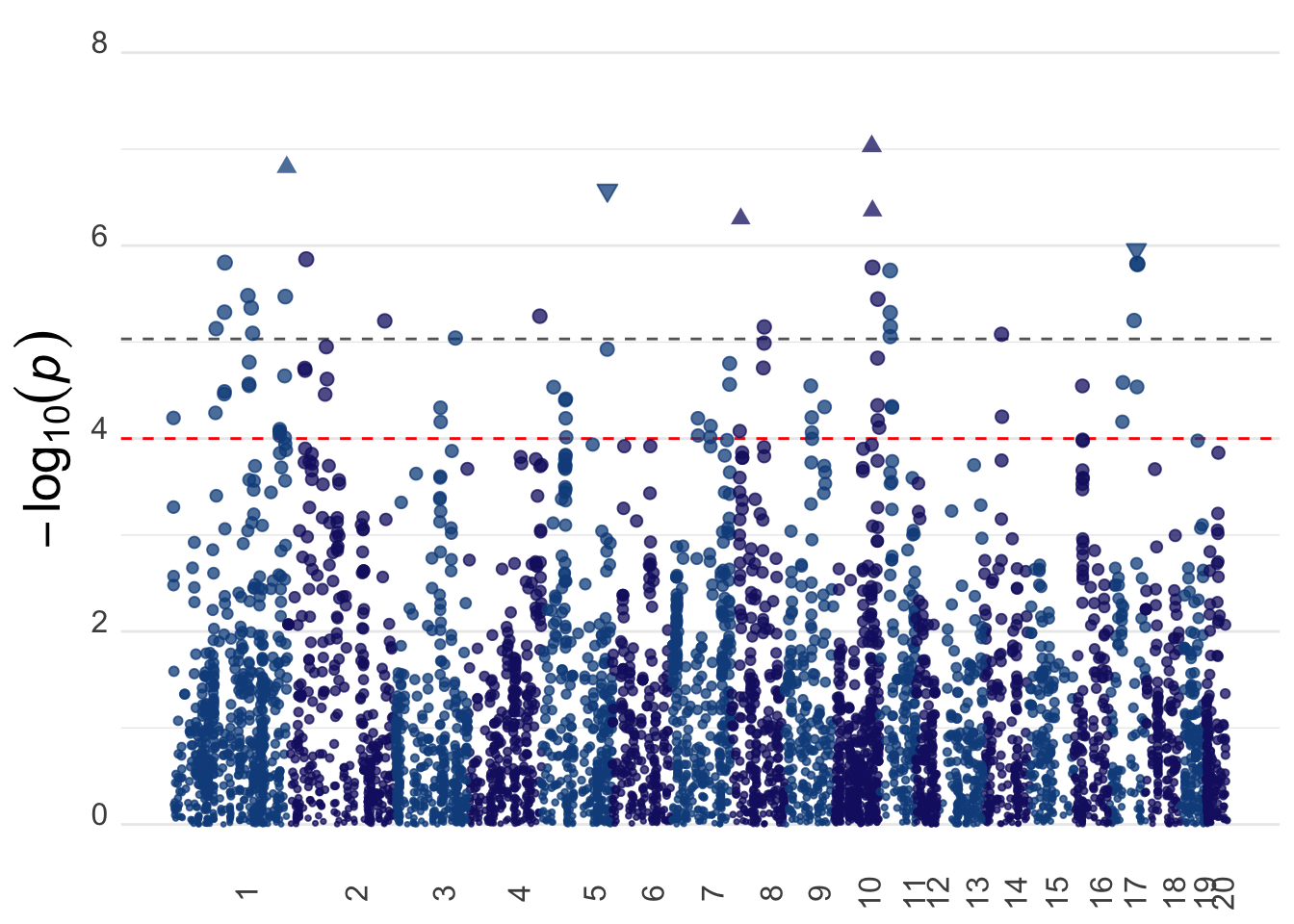
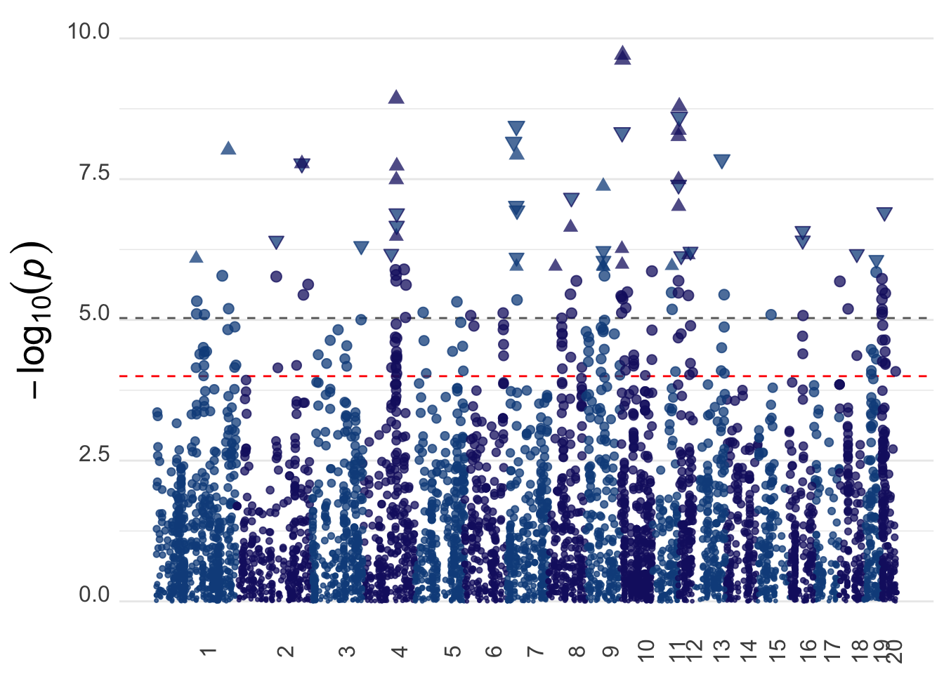
Generate Manhattan plots for BMI and height. If you wanted to add
labels for human genes, you can uncomment the
geom_label_repel line.
library(ggrepel)
data_cum <- bmi_manhat %>%
  group_by(chr) %>%
  summarise(max_bp = as.numeric(max(start))) %>%
  mutate(bp_add = lag(cumsum(max_bp), default = 0)) %>%
  select(chr, bp_add)
`summarise()` ungrouping output (override with `.groups` argument)gwas_data <- bmi_manhat %>%
inner_join(data_cum, by = "chr") %>%
mutate(bp_cum = start + bp_add)
axis_set <- gwas_data %>%
group_by(chr) %>%
summarize(center = mean(bp_cum))`summarise()` ungrouping output (override with `.groups` argument)ylim <- gwas_data %>%
filter(pvalue == min(pvalue)) %>%
mutate(ylim = abs(floor(log10(pvalue))) + 2) %>%
pull(ylim)
sig <- 0.05/(5388)
bmi_manhplot <- ggplot(gwas_data, aes(x = bp_cum, y = -log10(pvalue), color = as_factor(chr), size = -log10(pvalue))) +
geom_hline(yintercept = -log10(sig), color = "grey40", linetype = "dashed") +
geom_hline(yintercept = -log10(0.0001), color = "red", linetype = "dashed") +
geom_point(alpha = 0.75, shape = ifelse((gwas_data$zscore >= 4.863456), 17, ifelse(gwas_data$zscore <= -4.863456, 25, 19)), fill = "dodgerblue4") +
# geom_label_repel(aes(label=ifelse((pvalue <= sig & gene_name %in% human_bmi_genes$rat_gene), gene_name, "")), size = 6) +
ylim(c(0,8)) +
scale_x_continuous(label = axis_set$chr, breaks = axis_set$center) +
scale_color_manual(values = rep(c("dodgerblue4", "midnightblue"), unique(length(axis_set$chr)))) +
scale_size_continuous(range = c(0.5,3)) +
labs(x = NULL,
y = expression(-log[10](italic(p)))) +
theme_minimal() +
theme(
legend.position = "none",
panel.border = element_blank(),
panel.grid.major.x = element_blank(),
panel.grid.minor.x = element_blank(),
axis.text.x = element_text(angle = 90, size = 12),
axis.text.y = element_text( size = 12, vjust = 0),
axis.title = element_text(size = 20))
bmi_manhplotWarning: Removed 2 rows containing missing values (geom_point).
data_cum <- height_manhat %>%
  group_by(chr) %>%
  summarise(max_bp = as.numeric(max(start))) %>%
  mutate(bp_add = lag(cumsum(max_bp), default = 0)) %>%
  select(chr, bp_add)
`summarise()` ungrouping output (override with `.groups` argument)gwas_data <- height_manhat %>%
inner_join(data_cum, by = "chr") %>%
mutate(bp_cum = start + bp_add)
axis_set <- gwas_data %>%
group_by(chr) %>%
summarize(center = mean(bp_cum))`summarise()` ungrouping output (override with `.groups` argument)ylim <- gwas_data %>%
filter(pvalue == min(pvalue)) %>%
mutate(ylim = abs(floor(log10(pvalue))) + 2) %>%
pull(ylim)
sig <- 0.05/(5388)
height_manhplot <- ggplot(gwas_data, aes(x = bp_cum, y = -log10(pvalue),
color = as_factor(chr), size = -log10(pvalue))) +
geom_hline(yintercept = -log10(sig), color = "grey40", linetype = "dashed") +
geom_hline(yintercept = -log10(0.0001), color = "red", linetype = "dashed") +
geom_point(alpha = 0.75, shape = ifelse((gwas_data$zscore >= 4.863456), 17, ifelse(gwas_data$zscore <= -4.863456, 25, 19)), fill = "dodgerblue4") +
# geom_label_repel(aes(label=ifelse((pvalue <= sig & gene_name %in% human_height_genes$rat_gene), gene_name, "")), size = 6) +
ylim(c(0,10)) +
scale_x_continuous(label = axis_set$chr, breaks = axis_set$center) +
scale_color_manual(values = rep(c("dodgerblue4", "midnightblue"), unique(length(axis_set$chr)))) +
scale_size_continuous(range = c(0.5,3)) +
labs(x = NULL,
y = expression(-log[10](italic(p)))) +
theme_minimal() +
theme(
legend.position = "none",
panel.border = element_blank(),
panel.grid.major.x = element_blank(),
panel.grid.minor.x = element_blank(),
axis.text.x = element_text(angle = 90, size = 12),
axis.text.y = element_text( size = 12, vjust = 0),
axis.title = element_text(size = 20))
height_manhplotWarning: Removed 3 rows containing missing values (geom_point).
sessionInfo()R version 4.0.3 (2020-10-10)
Platform: x86_64-apple-darwin17.0 (64-bit)
Running under: macOS Big Sur 10.16
Matrix products: default
BLAS: /Library/Frameworks/R.framework/Versions/4.0/Resources/lib/libRblas.dylib
LAPACK: /Library/Frameworks/R.framework/Versions/4.0/Resources/lib/libRlapack.dylib
locale:
[1] en_US.UTF-8/en_US.UTF-8/en_US.UTF-8/C/en_US.UTF-8/en_US.UTF-8
attached base packages:
[1] stats graphics grDevices utils datasets methods base
other attached packages:
[1] ggrepel_0.9.1 forcats_0.5.0 stringr_1.4.0 dplyr_1.0.2
[5] purrr_0.3.4 tidyr_1.1.2 tibble_3.0.4 ggplot2_3.3.6
[9] tidyverse_1.3.0 readr_1.4.0
loaded via a namespace (and not attached):
[1] Rcpp_1.0.8.3 lubridate_1.7.9 assertthat_0.2.1 rprojroot_1.3-2
[5] digest_0.6.27 utf8_1.1.4 R6_2.4.1 cellranger_1.1.0
[9] backports_1.1.10 reprex_0.3.0 evaluate_0.15 highr_0.8
[13] httr_1.4.2 pillar_1.4.6 rlang_1.0.2 readxl_1.3.1
[17] rstudioapi_0.11 jquerylib_0.1.4 blob_1.2.1 rmarkdown_2.14
[21] labeling_0.4.2 munsell_0.5.0 broom_0.8.0 compiler_4.0.3
[25] httpuv_1.5.4 modelr_0.1.8 xfun_0.31 pkgconfig_2.0.3
[29] htmltools_0.5.2 tidyselect_1.1.0 workflowr_1.6.2 fansi_0.4.1
[33] crayon_1.3.4 dbplyr_1.4.4 withr_2.3.0 later_1.1.0.1
[37] grid_4.0.3 jsonlite_1.7.1 gtable_0.3.0 lifecycle_0.2.0
[41] DBI_1.1.0 git2r_0.27.1 magrittr_1.5 scales_1.1.1
[45] cli_3.3.0 stringi_1.5.3 farver_2.0.3 fs_1.5.0
[49] promises_1.1.1 xml2_1.3.2 bslib_0.3.1 ellipsis_0.3.2
[53] generics_0.0.2 vctrs_0.4.1 tools_4.0.3 glue_1.6.2
[57] hms_0.5.3 fastmap_1.1.0 yaml_2.2.1 colorspace_1.4-1
[61] rvest_0.3.6 knitr_1.39 haven_2.3.1 sass_0.4.1