Compare Gene Predictability and Heritability in Rat and Human Models
sabrina-mi
2022-08-23
Last updated: 2022-08-23
Checks: 6 1
Knit directory: RatXcan_Training/
This reproducible R Markdown analysis was created with workflowr (version 1.6.2). The Checks tab describes the reproducibility checks that were applied when the results were created. The Past versions tab lists the development history.
The R Markdown is untracked by Git. To know which version of the R
Markdown file created these results, you’ll want to first commit it to
the Git repo. If you’re still working on the analysis, you can ignore
this warning. When you’re finished, you can run
wflow_publish to commit the R Markdown file and build the
HTML.
Great job! The global environment was empty. Objects defined in the global environment can affect the analysis in your R Markdown file in unknown ways. For reproduciblity it’s best to always run the code in an empty environment.
The command set.seed(20220711) was run prior to running
the code in the R Markdown file. Setting a seed ensures that any results
that rely on randomness, e.g. subsampling or permutations, are
reproducible.
Great job! Recording the operating system, R version, and package versions is critical for reproducibility.
Nice! There were no cached chunks for this analysis, so you can be confident that you successfully produced the results during this run.
Great job! Using relative paths to the files within your workflowr project makes it easier to run your code on other machines.
Great! You are using Git for version control. Tracking code development and connecting the code version to the results is critical for reproducibility.
The results in this page were generated with repository version e8ceeb9. See the Past versions tab to see a history of the changes made to the R Markdown and HTML files.
Note that you need to be careful to ensure that all relevant files for
the analysis have been committed to Git prior to generating the results
(you can use wflow_publish or
wflow_git_commit). workflowr only checks the R Markdown
file, but you know if there are other scripts or data files that it
depends on. Below is the status of the Git repository when the results
were generated:
Ignored files:
    Ignored:    .Rhistory
    Ignored:    .Rproj.user/
    Ignored:    analysis/.Rhistory
    Ignored:    output/
    Ignored:    scripts/.Rhistory

Untracked files:
    Untracked:  .DS_Store
    Untracked:  .gitignore
    Untracked:  analysis/Plot_Predictability_Heritability.Rmd
    Untracked:  code/helpers.R

Unstaged changes:
    Modified:   analysis/.DS_Store
    Modified:   analysis/Analyze_PrediXcan_Results.Rmd
    Modified:   analysis/EN_Prediction_Model.Rmd
    Modified:   analysis/Run_PrediXcan.Rmd
    Modified:   analysis/index.Rmd
Note that any generated files, e.g. HTML, png, CSS, etc., are not included in this status report because it is ok for generated content to have uncommitted changes.
There are no past versions. Publish this analysis with
wflow_publish() to start tracking its development.
Previously, we computed heritability (h2) estimates for rat genes using GEMMA. And our PredictDB pipeline computes predictive performance (R2) for each gene when training the EN model. Now we compare it to heritability and predictability estimates for human genes generated by Wheeler Lab.
The sqlite database genarch.db
contains all results from Wheeler Lab’s multi-tissue analysis of GTEx
data. We queried R2 and h2 values and stored them in
human_h2.csv.
library(tidyverse)── Attaching packages ─────────────────────────────────────── tidyverse 1.3.0 ──✔ ggplot2 3.3.6 ✔ purrr 0.3.4
✔ tibble 3.0.4 ✔ dplyr 1.0.2
✔ tidyr 1.1.2 ✔ stringr 1.4.0
✔ readr 1.4.0 ✔ forcats 0.5.0── Conflicts ────────────────────────────────────────── tidyverse_conflicts() ──
✖ dplyr::filter() masks stats::filter()
✖ dplyr::lag() masks stats::lag()library(RSQLite)
"%&%" = function(a,b) paste(a,b,sep="")
dir = "/Users/sabrinami/Library/CloudStorage/Box-Box/imlab-data/data-Github/Rat_Genomics_Paper_Pipeline/"We first read in heritability estimes for humans and rats, and output their summary.
rat_h2 <- suppressMessages(read_tsv(dir %&% "GEMMA/Ac/Ac_PVE_estimates.txt", col_names = FALSE)) %>% dplyr::rename(rat_herit = X2)

human_h2_file = dir %&% "data/genarch.db"
sqlite.driver <- dbDriver("SQLite")
conn <- dbConnect(RSQLite::SQLite(), human_h2_file)
human_h2 <- dbGetQuery(conn, "select gene, ensid, en_r2 ,h2,h2_ci from results where tissue = 'DGN-WB'")
Warning in result_fetch(res@ptr, n = n): Column `en_r2`: mixed type, first seen
values of type real, coercing other values of type stringdbDisconnect(conn)
#remove ensembl version
human_h2$ensid <- sapply(strsplit(human_h2$ensid, "\\."), `[`, 1)
print("Distribution of Rat Gene Heritability")[1] "Distribution of Rat Gene Heritability"summary(rat_h2$rat_herit) Min. 1st Qu. Median Mean 3rd Qu. Max. NA's
0.02234 0.04492 0.06520 0.09822 0.11071 0.79924 58 print("Distribution of Human Gene Heritability")[1] "Distribution of Human Gene Heritability"summary(human_h2$h2) Min. 1st Qu. Median Mean 3rd Qu. Max.
0.000001 0.014847 0.057980 0.126364 0.173627 0.933770 Use the rat-human gene dictionary to join the two tables, and calculate the correlation of heritability for rats and humans.
orth.rats <- read_tsv(dir %&% "data/expression/ortholog_genes_rats_humans.tsv")
── Column specification ────────────────────────────────────────────────────────
cols(
  ensembl_gene_id = col_character(),
  external_gene_name = col_character(),
  rnorvegicus_homolog_ensembl_gene = col_character(),
  rnorvegicus_homolog_associated_gene_name = col_character()
)
rat_h2 <- rat_h2 %>% mutate(ensid = orth.rats[match(rat_h2$X1, orth.rats$rnorvegicus_homolog_ensembl_gene), 1]$ensembl_gene_id)
all_h2 <- inner_join(rat_h2, human_h2, by = "ensid")
cor.test(all_h2$rat_herit, all_h2$h2)
    Pearson's product-moment correlation

data:  all_h2$rat_herit and all_h2$h2
t = 6.9336, df = 10531, p-value = 4.344e-12
alternative hypothesis: true correlation is not equal to 0
95 percent confidence interval:
 0.04837588 0.08639778
sample estimates:
      cor
0.0674113
Repeat for predictability.
file <- dir %&% "Results/sql/Ac_output_db.db"
conn <- dbConnect(RSQLite::SQLite(), file)
rat_r2 <- dbGetQuery(conn, 'select * from extra')
dbDisconnect(conn)

rat_r2 <- rat_r2 %>% mutate(ensid = orth.rats[match(rat_r2$gene, orth.rats$rnorvegicus_homolog_ensembl_gene), 1]$ensembl_gene_id)
all_r2 <- inner_join(rat_r2, human_h2, by = "ensid")
cor.test(all_r2$R2, all_r2$en_r2)
    Pearson's product-moment correlation

data:  all_r2$R2 and all_r2$en_r2
t = 4.5828, df = 6068, p-value = 4.681e-06
alternative hypothesis: true correlation is not equal to 0
95 percent confidence interval:
 0.03362123 0.08376302
sample estimates:
       cor
0.05872917
Ac_h2 <- rat_h2 %>% dplyr::rename(gene.x = X1) %>% mutate(rat_ci = paste(round(rat_h2$X3, digits = 5), round(rat_h2$X4, digits = 5), sep = "-")) %>% dplyr::select(c(gene.x, rat_herit, rat_ci))
lg_df <- inner_join(all_r2, Ac_h2, by = "gene.x")
lg_df <- lg_df %>% dplyr::select(c(ensid, gene.x, genename, R2, en_r2,rat_herit,h2, rat_ci, h2_ci))
colnames(lg_df) = c("ensembl_id", "rat_ensembl_id", "genename", "rat_r2", "human_r2", "rat_h2", "human_h2", "rat_h2_ci", "human_h2_ci")Here we plot rat heritability against human heritability.
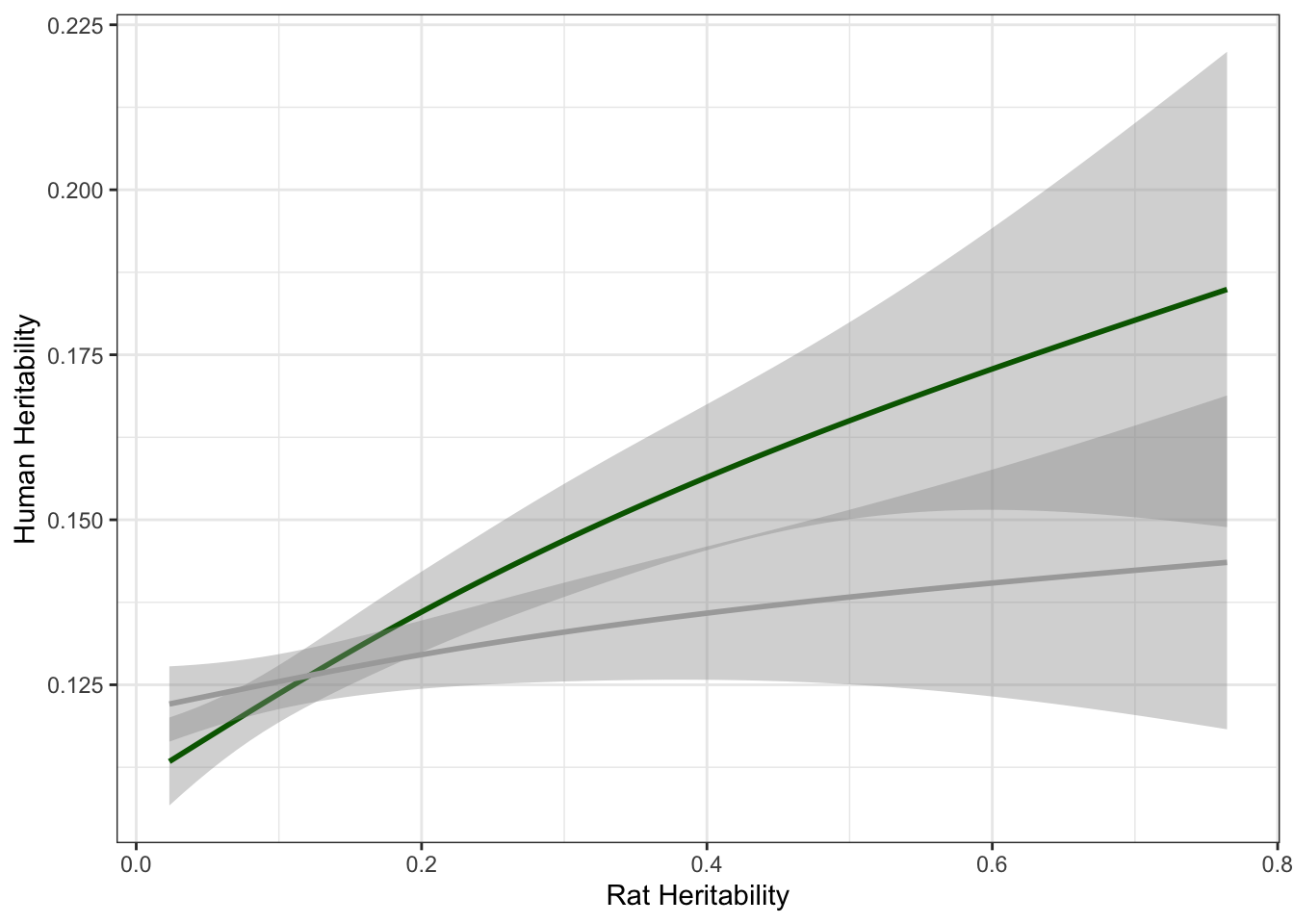
# Plot h2 between rats and Humans with line for null
lg_df %>% mutate(human_shuffled_h2 = sample(human_h2, nrow(lg_df), replace=F)) %>% ggplot(aes(rat_h2, human_h2)) + geom_smooth(col = "darkgreen") + geom_smooth(aes(rat_h2, human_shuffled_h2),col="dark gray")+theme_bw()+ xlab("Rat Heritability") + ylab("Human Heritability")
`geom_smooth()` using method = 'gam' and formula 'y ~ s(x, bs = "cs")'
`geom_smooth()` using method = 'gam' and formula 'y ~ s(x, bs = "cs")'
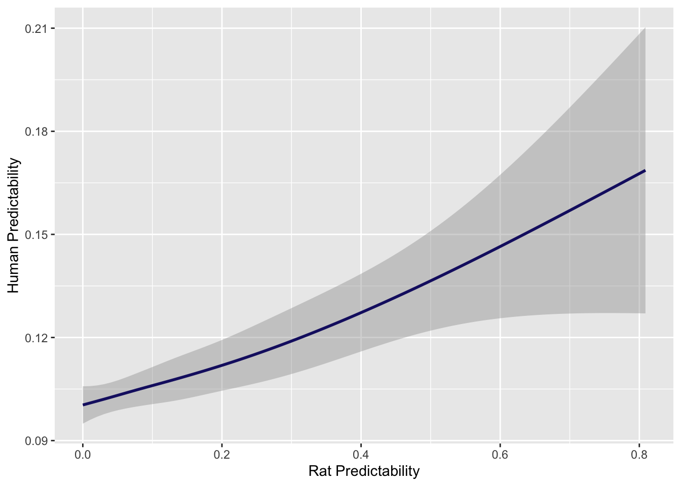
And repeat for predictability.
# Plot R2 between rats and Humans with line for null
lg_df %>% mutate(human_shuffled_r2 = sample(human_r2, nrow(lg_df), replace=F)) %>% ggplot(aes(rat_r2, human_r2)) + geom_smooth(col = "midnightblue") + xlab("Rat Predictability") + ylab("Human Predictability")
`geom_smooth()` using method = 'gam' and formula 'y ~ s(x, bs = "cs")'
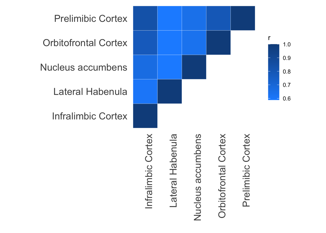
Plot correlation between predictability for every pair of tissues.
model.dir <- dir %&% "Results/sql/"
filelist <- c("Il_output_db.db", "Lh_output_db.db", "Ac_output_db.db", "Vo_output_db.db", "Pl_output_db.db")
tis.list <- c("Infralimbic Cortex", "Lateral Habenula", "Nucleus accumbens", "Orbitofrontal Cortex", "Prelimibic Cortex")

pred_tis <- data.frame(gene = as.character())
for(file in filelist) {
  filename <- model.dir %&% file
  print(filename)
  conn <- dbConnect(RSQLite::SQLite(), filename)
  i <- match(file, filelist)
  tis <- tis.list[i]
  extra <- dbGetQuery(conn, 'select * from extra') %>% select(c(gene, R2))
  colnames(extra)[2] = tis
  pred_tis <- full_join(pred_tis, extra, by = "gene")
  dbDisconnect(conn)
}
[1] "/Users/sabrinami/Library/CloudStorage/Box-Box/imlab-data/data-Github/Rat_Genomics_Paper_Pipeline/Results/sql/Il_output_db.db"
[1] "/Users/sabrinami/Library/CloudStorage/Box-Box/imlab-data/data-Github/Rat_Genomics_Paper_Pipeline/Results/sql/Lh_output_db.db"
[1] "/Users/sabrinami/Library/CloudStorage/Box-Box/imlab-data/data-Github/Rat_Genomics_Paper_Pipeline/Results/sql/Ac_output_db.db"
[1] "/Users/sabrinami/Library/CloudStorage/Box-Box/imlab-data/data-Github/Rat_Genomics_Paper_Pipeline/Results/sql/Vo_output_db.db"
[1] "/Users/sabrinami/Library/CloudStorage/Box-Box/imlab-data/data-Github/Rat_Genomics_Paper_Pipeline/Results/sql/Pl_output_db.db"rownames(pred_tis) <- pred_tis$gene
pred_tis <- pred_tis %>% select(-c(gene))
d1 <- cor(pred_tis %>% na.omit)
d1[lower.tri(d1)] <- NA
d1 <- d1 %>%
as.data.frame %>%
rownames_to_column(var = 'var1') %>%
gather(var2, value, -var1)
d1 <- d1 %>% dplyr::rename(r = value) %>% na.omit()
ggplot(data = d1, aes(x = var1, y = var2, fill = r)) +
geom_tile(color = "white")+
scale_fill_gradient(low="dodgerblue", high="dodgerblue4") +
theme_minimal() +
theme(panel.grid = element_blank()) + ylab("") + xlab("") + theme(axis.text = element_text(size = 15), axis.text.x = element_text(angle = 90, hjust = 1)) + theme(aspect.ratio=1) 
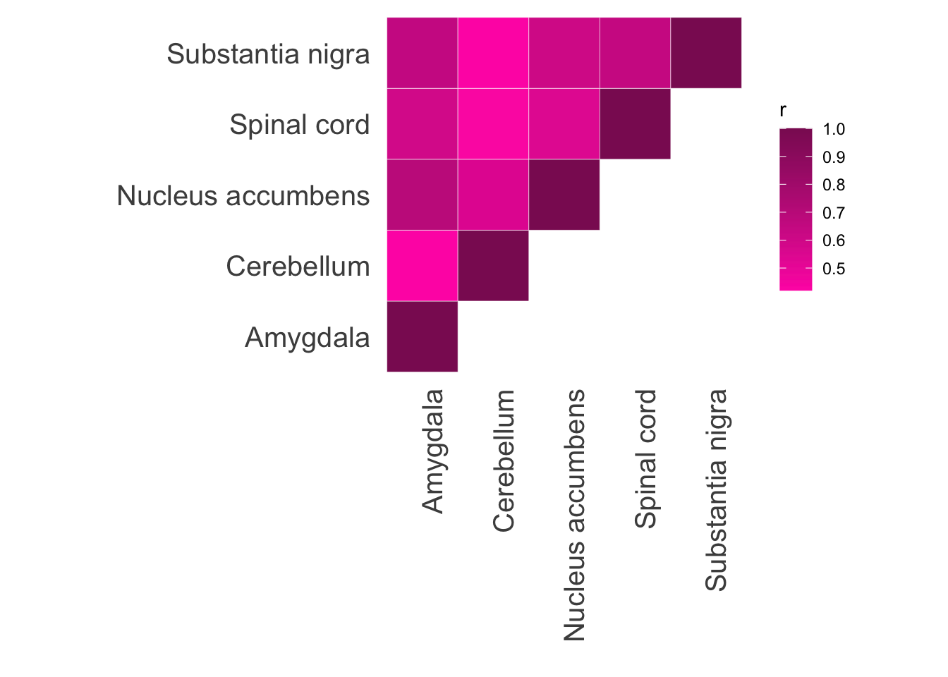
Repeat for analogous GTEx tissues. These EN models can be downloaded from PredictDB.
model.dir <- "~/elastic_net_models/"
tis.list = c("Amygdala", "Cerebellum", "Nucleus accumbens",  "Spinal cord", "Substantia nigra")
filelist <- c("en_Brain_Amygdala.db", "en_Brain_Cerebellum.db", "en_Brain_Nucleus_accumbens_basal_ganglia.db", "en_Brain_Spinal_cord_cervical_c-1.db", "en_Brain_Substantia_nigra.db")
pred_tis <- data.frame(gene = as.character())
for(file in filelist) {
filename <- model.dir %&% file
conn <- dbConnect(RSQLite::SQLite(), filename)
i <- match(file, filelist)
tis <- tis.list[i]
extra <- dbGetQuery(conn, 'select * from extra') %>% select(c(gene, pred.perf.R2))
colnames(extra)[2] = tis
pred_tis <- full_join(pred_tis, extra, by = "gene")
dbDisconnect(conn)
}
rownames(pred_tis) <- pred_tis$gene
pred_tis <- pred_tis %>% select(-c(gene))
d2 <- cor(pred_tis %>% na.omit)
d2[lower.tri(d2)] <- NA
d2 <- d2 %>%
as.data.frame %>%
rownames_to_column(var = 'var1') %>%
gather(var2, value, -var1)
d2 <- d2 %>% dplyr::rename(r = value) %>% na.omit()
ggplot(data = d2, aes(x = var1, y = var2, fill = r)) +
geom_tile(color = "white")+
scale_fill_gradient(low="maroon1", high="maroon4") +
theme_minimal() +
theme(panel.grid = element_blank()) + ylab("") + xlab("") + theme(axis.text = element_text(size = 15), axis.text.x = element_text(angle = 90, hjust = 1)) + theme(aspect.ratio=1) 
Compare number of SNPs used in prediction model for rats and humans.
summary(rat_r2$n.snps) Min. 1st Qu. Median Mean 3rd Qu. Max.
1.00 5.00 9.00 11.93 16.00 77.00 #human NAcc models
filename <- "~/elastic_net_models/en_Brain_Nucleus_accumbens_basal_ganglia.db"
sqlite.driver <- dbDriver("SQLite")
conn <- dbConnect(RSQLite::SQLite(), filename)
human_r2 <- dbGetQuery(conn, 'select * from extra')
summary(human_r2$n.snps.in.model) Min. 1st Qu. Median Mean 3rd Qu. Max.
1.00 13.00 24.00 31.08 42.00 226.00
sessionInfo()R version 4.0.3 (2020-10-10)
Platform: x86_64-apple-darwin17.0 (64-bit)
Running under: macOS Big Sur 10.16
Matrix products: default
BLAS: /Library/Frameworks/R.framework/Versions/4.0/Resources/lib/libRblas.dylib
LAPACK: /Library/Frameworks/R.framework/Versions/4.0/Resources/lib/libRlapack.dylib
locale:
[1] en_US.UTF-8/en_US.UTF-8/en_US.UTF-8/C/en_US.UTF-8/en_US.UTF-8
attached base packages:
[1] stats graphics grDevices utils datasets methods base
other attached packages:
[1] RSQLite_2.2.1 forcats_0.5.0 stringr_1.4.0 dplyr_1.0.2
[5] purrr_0.3.4 readr_1.4.0 tidyr_1.1.2 tibble_3.0.4
[9] ggplot2_3.3.6 tidyverse_1.3.0
loaded via a namespace (and not attached):
[1] Rcpp_1.0.8.3 lattice_0.20-41 lubridate_1.7.9 assertthat_0.2.1
[5] rprojroot_1.3-2 digest_0.6.27 R6_2.4.1 cellranger_1.1.0
[9] backports_1.1.10 reprex_0.3.0 evaluate_0.15 highr_0.8
[13] httr_1.4.2 pillar_1.4.6 rlang_1.0.2 readxl_1.3.1
[17] rstudioapi_0.11 jquerylib_0.1.4 blob_1.2.1 Matrix_1.2-18
[21] rmarkdown_2.14 labeling_0.4.2 splines_4.0.3 bit_4.0.4
[25] munsell_0.5.0 broom_0.8.0 compiler_4.0.3 httpuv_1.5.4
[29] modelr_0.1.8 xfun_0.31 pkgconfig_2.0.3 mgcv_1.8-33
[33] htmltools_0.5.2 tidyselect_1.1.0 workflowr_1.6.2 crayon_1.3.4
[37] dbplyr_1.4.4 withr_2.3.0 later_1.1.0.1 grid_4.0.3
[41] nlme_3.1-150 jsonlite_1.7.1 gtable_0.3.0 lifecycle_0.2.0
[45] DBI_1.1.0 git2r_0.27.1 magrittr_1.5 scales_1.1.1
[49] cli_3.3.0 stringi_1.5.3 farver_2.0.3 fs_1.5.0
[53] promises_1.1.1 xml2_1.3.2 bslib_0.3.1 ellipsis_0.3.2
[57] generics_0.0.2 vctrs_0.4.1 tools_4.0.3 bit64_4.0.5
[61] glue_1.6.2 hms_1.1.2 fastmap_1.1.0 yaml_2.2.1
[65] colorspace_1.4-1 rvest_0.3.6 memoise_1.1.0 knitr_1.39
[69] haven_2.3.1 sass_0.4.1