Figure 1
Last updated: 2021-07-06
Checks: 6 1
Knit directory: scRNA_NB_comparison/
This reproducible R Markdown analysis was created with workflowr (version 1.6.2). The Checks tab describes the reproducibility checks that were applied when the results were created. The Past versions tab lists the development history.
The R Markdown is untracked by Git. To know which version of the R Markdown file created these results, you’ll want to first commit it to the Git repo. If you’re still working on the analysis, you can ignore this warning. When you’re finished, you can run wflow_publish to commit the R Markdown file and build the HTML.
Great job! The global environment was empty. Objects defined in the global environment can affect the analysis in your R Markdown file in unknown ways. For reproduciblity it’s best to always run the code in an empty environment.
The command set.seed(20210706) was run prior to running the code in the R Markdown file. Setting a seed ensures that any results that rely on randomness, e.g. subsampling or permutations, are reproducible.
Great job! Recording the operating system, R version, and package versions is critical for reproducibility.
Nice! There were no cached chunks for this analysis, so you can be confident that you successfully produced the results during this run.
Great job! Using relative paths to the files within your workflowr project makes it easier to run your code on other machines.
Great! You are using Git for version control. Tracking code development and connecting the code version to the results is critical for reproducibility.
The results in this page were generated with repository version e0b7c2c. See the Past versions tab to see a history of the changes made to the R Markdown and HTML files.
Note that you need to be careful to ensure that all relevant files for the analysis have been committed to Git prior to generating the results (you can use wflow_publish or wflow_git_commit). workflowr only checks the R Markdown file, but you know if there are other scripts or data files that it depends on. Below is the status of the Git repository when the results were generated:
Ignored files:
    Ignored:    data/raw_data/
    Ignored:    data/rds_filtered/
    Ignored:    data/rds_raw/
    Ignored:    output/snakemake_output/

Untracked files:
    Untracked:  analysis/01_Smart-seq3.Rmd
    Untracked:  analysis/02_Mereu.Rmd
    Untracked:  analysis/03A_Ding-Mixture-HEK-3T3.Rmd
    Untracked:  analysis/03B_Ding-PBMC.Rmd
    Untracked:  analysis/03C_Ding-Cortex.Rmd
    Untracked:  analysis/04_PBMC68k.Rmd
    Untracked:  analysis/05_Fetal-sciRNAseq3.Rmd
    Untracked:  analysis/06G_VS2020_Seurat.Rmd
    Untracked:  analysis/07_Filter_all_datasets.Rmd
    Untracked:  analysis/08_Downsample_PBMC__Smart-seq3.Rmd
    Untracked:  analysis/09_Figure1.Rmd
    Untracked:  analysis/10_Figure2.Rmd
    Untracked:  analysis/11_Figure3.Rmd
    Untracked:  analysis/12_SuppFigure-DataStats.Rmd
    Untracked:  analysis/13_SuppFigure-VST.Rmd
    Untracked:  analysis/14_SuppFigure-Simulation.Rmd
    Untracked:  analysis/15_SuppFigure-Upsampling.Rmd
    Untracked:  data/datasets.csv
    Untracked:  data/sampled_counts/

Unstaged changes:
    Modified:   .gitignore
    Modified:   analysis/_site.yml
    Modified:   analysis/about.Rmd
    Modified:   analysis/index.Rmd
    Modified:   analysis/license.Rmd
Note that any generated files, e.g. HTML, png, CSS, etc., are not included in this status report because it is ok for generated content to have uncommitted changes.
There are no past versions. Publish this analysis with wflow_publish() to start tracking its development.
Read datassets
datasets <- readr::read_csv(here::here("data", "datasets.csv"), col_types = readr::cols())
datasets$datatype <- factor(datasets$datatype, levels = c("technical-control", "cell line", "heterogeneous"))
datasets <- datasets %>% arrange(datatype)
Read and process poisson GLM results
QVALUE_THRESHOLD <- 1e-2
ncells <- "1000"
residual_type <- "quantile"
nb_column <- paste0("qval_ssr", "_", residual_type)
ssr_column <- paste0("ssr", "_", residual_type, "_normalized")
root_dir <- here::here("output/snakemake_output/poisson_glm_output", ncells)


fits <- GetFits(root_dir, qval_col = nb_column)
fits_dfx <- fits[["fits"]]
frac_dfx <- fits[["frac_df"]]
cell_attrs <- fits[["cell_attrs"]]
gene_attrs <- fits[["gene_attrs"]]

fits_df <- ProcessFits(fits_dfx, datasets, nb_column)
frac_df <- left_join(frac_dfx, datasets, by = "key")
Fraction of non-poisson genes
frac_df_subset <- frac_df[, c(
  "sample_name", "datatype",
  "median_gene_avg_umi", "median_cell_total_umi", "nonpoisson_fraction"
)] %>% arrange(nonpoisson_fraction)
frac_df_subset <- frac_df_subset %>% mutate(across(where(is.numeric), round, 3))
kbl(frac_df_subset, booktabs = T) %>%
kable_styling(latex_options = "striped")| sample_name | datatype | median_gene_avg_umi | median_cell_total_umi | nonpoisson_fraction |
|---|---|---|---|---|
| TechCtrl1 (ChromiumV1) | technical-control | 0.007 | 2264.5 | 0.001 |
| TechCtrl2 (ChromiumV1) | technical-control | 0.007 | 2165.0 | 0.004 |
| TechCtrl (inDrops) | technical-control | 0.365 | 32905.0 | 0.005 |
| PBMC-r2 (Seq-Well) | heterogeneous | 0.009 | 521.0 | 0.007 |
| HEK-m (ChromiumV2_sn) | cell line | 0.171 | 4967.0 | 0.008 |
| PBMC-r1 (inDrops) | heterogeneous | 0.010 | 798.0 | 0.009 |
| HEK-m (inDrops) | cell line | 0.108 | 2943.0 | 0.010 |
| PBMC68k (ChromiumV1) | heterogeneous | 0.011 | 1513.0 | 0.011 |
| PBMC-r1 (Drop-seq) | heterogeneous | 0.012 | 1554.5 | 0.015 |
| PBMC-r2 (CEL-seq2) | heterogeneous | 0.069 | 5917.0 | 0.016 |
| PBMC-r2 (ChromiumV2) | heterogeneous | 0.021 | 2850.5 | 0.016 |
| HEK-r1 (inDrops) | cell line | 0.042 | 3132.0 | 0.017 |
| PBMC-r1 (Seq-Well) | heterogeneous | 0.011 | 1200.0 | 0.017 |
| PBMC-r1 (ChromiumV2A) | heterogeneous | 0.016 | 2384.0 | 0.018 |
| PBMC-r2 (inDrops) | heterogeneous | 0.018 | 1690.0 | 0.019 |
| PBMC-r1 (ChromiumV2B) | heterogeneous | 0.019 | 3286.0 | 0.020 |
| PBMC-r1 (CEL-seq2) | heterogeneous | 0.071 | 6848.0 | 0.021 |
| HEK-r2 (inDrops) | cell line | 0.052 | 3973.0 | 0.027 |
| 3T3-r1 (inDrops) | cell line | 0.051 | 2255.0 | 0.027 |
| PBMC-r2 (Drop-seq) | heterogeneous | 0.017 | 2486.5 | 0.028 |
| 3T3-r2 (Drop-seq) | cell line | 0.080 | 3434.0 | 0.031 |
| Cortex-r2 (ChromiumV2) | heterogeneous | 0.042 | 3980.5 | 0.036 |
| 3T3-r1 (Drop-seq) | cell line | 0.072 | 3152.5 | 0.038 |
| HEK-r1 (Drop-seq) | cell line | 0.053 | 6015.5 | 0.039 |
| HEK-r2 (Drop-seq) | cell line | 0.048 | 6312.5 | 0.040 |
| 3T3-r2 (inDrops) | cell line | 0.107 | 4666.5 | 0.041 |
| Cortex-r2 (sci-RNA-seq) | heterogeneous | 0.029 | 3501.5 | 0.046 |
| PBMC-r1 (ChromiumV3) | heterogeneous | 0.029 | 5839.5 | 0.046 |
| Cortex-r1 (DroNc-seq) | heterogeneous | 0.043 | 3013.5 | 0.050 |
| 3T3-r1 (sci-RNA-seq) | cell line | 0.188 | 6609.5 | 0.061 |
| PBMC (ChromiumV3) | heterogeneous | 0.050 | 6992.0 | 0.064 |
| 3T3 (ChromiumV3) | cell line | 0.072 | 16184.5 | 0.066 |
| Cortex-r2 (DroNc-seq) | heterogeneous | 0.050 | 3094.0 | 0.068 |
| Cortex-r1 (ChromiumV2) | heterogeneous | 0.065 | 7132.5 | 0.071 |
| HEK-r1 (sci-RNA-seq) | cell line | 0.220 | 11490.0 | 0.072 |
| Cortex-r1 (sci-RNA-seq) | heterogeneous | 0.031 | 4421.0 | 0.074 |
| HEK (ChromiumV3) | cell line | 0.069 | 41054.5 | 0.116 |
| HEK-m (Drop-seq) | cell line | 0.109 | 1907.5 | 0.116 |
| HEK-m (MARS-seq) | cell line | 0.235 | 11207.5 | 0.131 |
| Fetal (sci-RNA-seq3) | heterogeneous | 0.030 | 6975.5 | 0.134 |
| 3T3-r2 (ChromiumV2) | cell line | 0.185 | 14057.0 | 0.141 |
| 3T3-r1 (ChromiumV2) | cell line | 0.151 | 11834.0 | 0.143 |
| 3T3-r2 (sci-RNA-seq) | cell line | 0.161 | 9199.0 | 0.150 |
| HEK-r2 (sci-RNA-seq) | cell line | 0.096 | 13298.0 | 0.152 |
| HEK-r2 (CEL-seq2) | cell line | 0.389 | 43670.0 | 0.158 |
| HEK-r1 (CEL-seq2) | cell line | 0.615 | 52973.0 | 0.160 |
| HEK-r1 (ChromiumV2) | cell line | 0.108 | 25193.5 | 0.164 |
| HEK-r2 (ChromiumV2) | cell line | 0.096 | 23444.0 | 0.168 |
| 3T3-r1 (CEL-seq2) | cell line | 0.616 | 34291.0 | 0.172 |
| HEK-m (mcSCRB-seq) | cell line | 0.121 | 3266.5 | 0.176 |
| 3T3-r2 (CEL-seq2) | cell line | 1.045 | 53036.0 | 0.220 |
| HEK (Smart-seq3) | cell line | 0.286 | 106996.0 | 0.233 |
| HEK-m (CEL-seq2) | cell line | 0.788 | 60592.5 | 0.242 |
| PBMC (Smart-seq3) | heterogeneous | 0.032 | 9487.5 | 0.396 |
| HEK-m (ddSeq) | cell line | 0.205 | 5304.5 | 0.570 |
| HEK-m (ChromiumV2) | cell line | 0.710 | 73333.5 | 0.617 |
| Fibroblasts (Smart-seq3) | heterogeneous | 0.526 | 197151.0 | 0.627 |
| HEK-m (Quartz-Seq2) | cell line | 1.576 | 167199.0 | 0.643 |
dir.create(here::here("output", "tables"), showWarnings = F)
print(xtable(frac_df_subset, type = "latex",  digits=3), include.rownames = FALSE, file = here::here("output/tables/fraction_nonpoisson.tex"))
Medium to high mean non-poisson genes
medium_high_gene_pois <- list()
for (sample_name in unique(fits_df$sample_name)) {
  df <- fits_df[fits_df$sample_name == sample_name, ]

  med_abundance <- df[(df$mean > 1),]# & (df$mean <= 10), ]
  med_abundance_nonpois <- med_abundance[med_abundance$gene_type != "Pass", ]

  ratio <- dim(med_abundance_nonpois)[1] / dim(med_abundance)[1]

  medium_high_gene_pois[[sample_name]] <- data.frame(ratio = ratio, n_med_high_nonpoisson = dim(med_abundance_nonpois)[1], n_med_high = dim(med_abundance)[1], n_all = dim(df)[1])
}
medium_high_gene_pois <- bind_rows(medium_high_gene_pois, .id = "sample_name")

kbl(medium_high_gene_pois, booktabs = T) %>%
kable_styling(latex_options = "striped")| sample_name | ratio | n_med_high_nonpoisson | n_med_high | n_all |
|---|---|---|---|---|
| TechCtrl1 (ChromiumV1) | 0.1200000 | 18 | 150 | 20167 |
| TechCtrl2 (ChromiumV1) | 0.5942029 | 82 | 138 | 20838 |
| TechCtrl (inDrops) | 0.0248205 | 159 | 6406 | 25255 |
| 3T3 (ChromiumV3) | 0.5739750 | 1288 | 2244 | 21920 |
| 3T3-r1 (CEL-seq2) | 0.4772430 | 2915 | 6108 | 15457 |
| 3T3-r1 (ChromiumV2) | 0.8469945 | 1550 | 1830 | 15390 |
| 3T3-r1 (Drop-seq) | 0.6404293 | 358 | 559 | 13904 |
| 3T3-r1 (inDrops) | 0.8095238 | 238 | 294 | 13337 |
| 3T3-r1 (sci-RNA-seq) | 0.5337150 | 839 | 1572 | 12806 |
| 3T3-r2 (CEL-seq2) | 0.5292932 | 3939 | 7442 | 14620 |
| 3T3-r2 (ChromiumV2) | 0.7796818 | 1911 | 2451 | 15127 |
| 3T3-r2 (Drop-seq) | 0.5175953 | 353 | 682 | 13977 |
| 3T3-r2 (inDrops) | 0.5410200 | 488 | 902 | 12354 |
| 3T3-r2 (sci-RNA-seq) | 0.8837209 | 1824 | 2064 | 15608 |
| HEK (ChromiumV3) | 0.6252152 | 3268 | 5227 | 26012 |
| HEK (Smart-seq3) | 0.7991825 | 7625 | 9541 | 27097 |
| HEK-r1 (CEL-seq2) | 0.5020683 | 4248 | 8461 | 19628 |
| HEK-r1 (ChromiumV2) | 0.8846924 | 3092 | 3495 | 21809 |
| HEK-r1 (Drop-seq) | 0.5256125 | 708 | 1347 | 19149 |
| HEK-r1 (inDrops) | 0.6119048 | 257 | 420 | 17091 |
| HEK-r1 (sci-RNA-seq) | 0.5555202 | 1746 | 3143 | 17299 |
| HEK-r2 (CEL-seq2) | 0.5539335 | 4098 | 7398 | 20294 |
| HEK-r2 (ChromiumV2) | 0.9304878 | 3052 | 3280 | 22655 |
| HEK-r2 (Drop-seq) | 0.6598891 | 714 | 1082 | 20614 |
| HEK-r2 (inDrops) | 0.6548387 | 406 | 620 | 17862 |
| HEK-r2 (sci-RNA-seq) | 0.9221675 | 2808 | 3045 | 23608 |
| HEK-m (CEL-seq2) | 0.6930805 | 6761 | 9755 | 21665 |
| HEK-m (ChromiumV2) | 0.9761956 | 9063 | 9284 | 21669 |
| HEK-m (ChromiumV2_sn) | 0.1847826 | 153 | 828 | 16502 |
| HEK-m (ddSeq) | 0.9952525 | 2306 | 2317 | 18354 |
| HEK-m (Drop-seq) | 0.9843505 | 629 | 639 | 15794 |
| HEK-m (inDrops) | 0.3333333 | 174 | 522 | 13118 |
| HEK-m (MARS-seq) | 0.8183222 | 1590 | 1943 | 18091 |
| HEK-m (mcSCRB-seq) | 0.9458333 | 1135 | 1200 | 13760 |
| HEK-m (Quartz-Seq2) | 0.9814356 | 11895 | 12120 | 21535 |
| Cortex-r1 (ChromiumV2) | 0.7914110 | 903 | 1141 | 22947 |
| Cortex-r1 (DroNc-seq) | 0.9180887 | 269 | 293 | 21965 |
| Cortex-r1 (sci-RNA-seq) | 0.9776248 | 568 | 581 | 22188 |
| Cortex-r2 (ChromiumV2) | 0.8245614 | 329 | 399 | 22920 |
| Cortex-r2 (DroNc-seq) | 0.9213251 | 445 | 483 | 21183 |
| Cortex-r2 (sci-RNA-seq) | 0.9878788 | 326 | 330 | 22492 |
| Fibroblasts (Smart-seq3) | 0.9940432 | 10680 | 10744 | 24003 |
| PBMC-r1 (CEL-seq2) | 0.4225513 | 371 | 878 | 19767 |
| PBMC-r1 (ChromiumV2A) | 0.9219512 | 189 | 205 | 21706 |
| PBMC-r1 (ChromiumV2B) | 0.8710801 | 250 | 287 | 21922 |
| PBMC-r1 (ChromiumV3) | 0.8385214 | 431 | 514 | 22851 |
| PBMC-r1 (Drop-seq) | 0.8555556 | 154 | 180 | 21292 |
| PBMC-r1 (inDrops) | 0.9696970 | 64 | 66 | 17972 |
| PBMC-r1 (Seq-Well) | 0.9624060 | 128 | 133 | 21785 |
| PBMC-r2 (CEL-seq2) | 0.4237288 | 275 | 649 | 19705 |
| PBMC-r2 (ChromiumV2) | 0.8448276 | 196 | 232 | 22283 |
| PBMC-r2 (Drop-seq) | 0.9432314 | 216 | 229 | 23577 |
| PBMC-r2 (inDrops) | 0.9754601 | 159 | 163 | 19143 |
| PBMC-r2 (Seq-Well) | 0.9411765 | 64 | 68 | 15088 |
| PBMC68k (ChromiumV1) | 0.8490566 | 135 | 159 | 19955 |
| PBMC (ChromiumV3) | 0.7309645 | 576 | 788 | 17853 |
| PBMC (Smart-seq3) | 0.9763514 | 1156 | 1184 | 28768 |
| Fetal (sci-RNA-seq3) | 0.7037037 | 19 | 27 | 46844 |
print(xtable(medium_high_gene_pois, digits=3), include.rownames = FALSE, digits=3, file = here::here("output/tables/medium_high_expr_nonpois_fraction.tex"))Plot fraction of non-poisson vs gene abundance
nonpoismeanwise <- GetMeanwiseNonPois(fits_df)
nonpoismeanwise <- left_join(nonpoismeanwise, datasets, by = "key")
nonpoismeanwise_df <- nonpoismeanwise[complete.cases(nonpoismeanwise), ]
nonpoismeanwise_df$sample_name <- factor(nonpoismeanwise_df$sample_name, levels = datasets$sample_name)

nonpoismeanwise_filtered <- nonpoismeanwise_df[nonpoismeanwise_df$n_total_genes >= 10, ]


plot.dots <- ggplot(nonpoismeanwise_filtered, aes(sample_name, mean_quantile,
  color = nonpoisson_fraction,
  size = nonpoisson_fraction
)) +
  geom_point() +
  scale_color_viridis_c(
    direction = -1,
    breaks = c(0.25, 0.5, 0.75, 1),
    name = "Non-poisson fraction"
  ) +
  scale_size(
    name = "Non-poisson fraction",
    breaks = c(0.25, 0.5, 0.75, 1),
    range = c(0.5, 5)
  ) +
  theme_pubr(base_size = 10) +
  theme(legend.position = "right", legend.direction = "horizontal") +
  guides(color = guide_legend(), size = guide_legend()) +
  guides(x = guide_axis(angle = 90)) +
  xlab("") +
  ylab("Gene mean") +
  theme(legend.position = c(0.8, 1.05))

plot.dots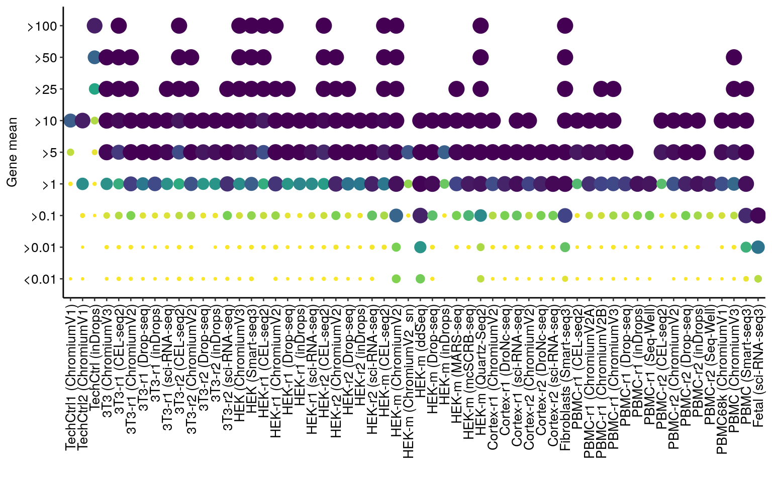
nonpoismeanwise_filtered_subset <- nonpoismeanwise_filtered[, c("sample_name", "mean_quantile", "nonpoisson_fraction")]
nonpoismeanwise_filtered_subset2 <- tidyr::spread(nonpoismeanwise_filtered_subset, mean_quantile, nonpoisson_fraction)

kbl(nonpoismeanwise_filtered_subset2, booktabs = T) %>%
kable_styling(latex_options = "striped")| sample_name | <0.01 | >0.01 | >0.1 | >1 | >5 | >10 | >25 | >50 | >100 |
|---|---|---|---|---|---|---|---|---|---|
| TechCtrl1 (ChromiumV1) | 0.0001579 | NA | NA | 0.0083333 | 0.1000000 | 0.7000000 | NA | NA | NA |
| TechCtrl2 (ChromiumV1) | 0.0002289 | 0.0001568 | 0.0181219 | 0.5090909 | NA | 0.9285714 | NA | NA | NA |
| TechCtrl (inDrops) | NA | NA | 0.0002956 | 0.0051442 | 0.0369069 | 0.1264822 | 0.4102564 | 0.6734694 | 0.9285714 |
| 3T3 (ChromiumV3) | 0.0016598 | 0.0071594 | 0.0664159 | 0.4941676 | 0.9889503 | 1.0000000 | 1.0000000 | 1.0000000 | NA |
| 3T3-r1 (CEL-seq2) | 0.0071702 | 0.0073620 | 0.1178304 | 0.3713582 | 0.8368984 | 0.9785933 | 1.0000000 | 1.0000000 | 1.0000000 |
| 3T3-r1 (ChromiumV2) | 0.0044398 | 0.0108141 | 0.1958763 | 0.8197038 | 1.0000000 | 1.0000000 | 1.0000000 | 1.0000000 | NA |
| 3T3-r1 (Drop-seq) | 0.0015552 | 0.0006245 | 0.0542621 | 0.6019802 | 1.0000000 | 1.0000000 | NA | NA | NA |
| 3T3-r1 (inDrops) | 0.0008782 | 0.0010646 | 0.0463543 | 0.7786561 | 1.0000000 | 1.0000000 | NA | NA | NA |
| 3T3-r1 (sci-RNA-seq) | 0.0007918 | 0.0033213 | 0.0558642 | 0.4965612 | 0.9873418 | 1.0000000 | 1.0000000 | NA | NA |
| 3T3-r2 (CEL-seq2) | 0.0075930 | 0.0091783 | 0.1038343 | 0.3863328 | 0.7697466 | 0.9505247 | 1.0000000 | 1.0000000 | 1.0000000 |
| 3T3-r2 (ChromiumV2) | 0.0081105 | 0.0062435 | 0.1431002 | 0.7383721 | 1.0000000 | 1.0000000 | 1.0000000 | 1.0000000 | NA |
| 3T3-r2 (Drop-seq) | 0.0012251 | NA | 0.0386980 | 0.4691558 | 0.9534884 | 1.0000000 | NA | NA | NA |
| 3T3-r2 (inDrops) | 0.0009862 | 0.0005052 | 0.0289113 | 0.4843554 | 0.9710145 | 1.0000000 | NA | NA | NA |
| 3T3-r2 (sci-RNA-seq) | 0.0048852 | 0.0075633 | 0.2089249 | 0.8717263 | 1.0000000 | 1.0000000 | 1.0000000 | NA | NA |
| HEK (ChromiumV3) | 0.0030717 | 0.0063885 | 0.0762431 | 0.5129495 | 0.9671642 | 1.0000000 | 1.0000000 | 1.0000000 | 1.0000000 |
| HEK (Smart-seq3) | 0.0124555 | 0.0121248 | 0.1717452 | 0.7031738 | 0.9428066 | 0.9871324 | 1.0000000 | 1.0000000 | 1.0000000 |
| HEK-r1 (CEL-seq2) | NA | 0.0084314 | 0.0921942 | 0.3756942 | 0.7605156 | 0.9398734 | 1.0000000 | 1.0000000 | 1.0000000 |
| HEK-r1 (ChromiumV2) | 0.0054479 | 0.0179791 | 0.1583698 | 0.8531876 | 1.0000000 | 1.0000000 | 1.0000000 | NA | 1.0000000 |
| HEK-r1 (Drop-seq) | 0.0004613 | 0.0029189 | 0.0376685 | 0.4732069 | 1.0000000 | 1.0000000 | 1.0000000 | NA | NA |
| HEK-r1 (inDrops) | 0.0005487 | 0.0011022 | 0.0197816 | 0.5421348 | 1.0000000 | 1.0000000 | NA | NA | NA |
| HEK-r1 (sci-RNA-seq) | 0.0047764 | 0.0069048 | 0.0763099 | 0.5151621 | 0.9710145 | 1.0000000 | NA | NA | NA |
| HEK-r2 (CEL-seq2) | 0.0051769 | 0.0080345 | 0.0847489 | 0.4479185 | 0.9014228 | 0.9844098 | 1.0000000 | 1.0000000 | 1.0000000 |
| HEK-r2 (ChromiumV2) | 0.0055034 | 0.0191110 | 0.2030820 | 0.9113186 | 1.0000000 | 1.0000000 | 1.0000000 | 1.0000000 | NA |
| HEK-r2 (Drop-seq) | 0.0012235 | 0.0031302 | 0.0587045 | 0.6178609 | 1.0000000 | 1.0000000 | 1.0000000 | NA | NA |
| HEK-r2 (inDrops) | 0.0008364 | 0.0027337 | 0.0275229 | 0.6014898 | 1.0000000 | 1.0000000 | NA | NA | NA |
| HEK-r2 (sci-RNA-seq) | 0.0058964 | 0.0177192 | 0.2650504 | 0.9149013 | 1.0000000 | 1.0000000 | NA | NA | NA |
| HEK-m (CEL-seq2) | NA | 0.0187520 | 0.1357605 | 0.6062354 | 0.9279762 | 0.9898990 | 1.0000000 | 1.0000000 | 1.0000000 |
| HEK-m (ChromiumV2) | 0.1884058 | 0.2037037 | 0.6752822 | 0.9689714 | 0.9984825 | 1.0000000 | 1.0000000 | 1.0000000 | 1.0000000 |
| HEK-m (ChromiumV2_sn) | NA | NA | 0.0053493 | 0.1718171 | 0.7333333 | NA | NA | NA | NA |
| HEK-m (ddSeq) | 0.2215190 | 0.4792910 | 0.9116033 | 0.9945972 | 1.0000000 | 1.0000000 | NA | NA | NA |
| HEK-m (Drop-seq) | 0.0058252 | 0.0138690 | 0.2911326 | 0.9819820 | 1.0000000 | 1.0000000 | NA | NA | NA |
| HEK-m (inDrops) | NA | NA | 0.0078245 | 0.2494331 | 0.6909091 | 1.0000000 | NA | NA | NA |
| HEK-m (MARS-seq) | NA | 0.0101597 | 0.2094223 | 0.7965318 | 0.9916667 | 1.0000000 | 1.0000000 | NA | NA |
| HEK-m (mcSCRB-seq) | NA | 0.0069649 | 0.3341531 | 0.9397032 | 1.0000000 | 1.0000000 | NA | NA | NA |
| HEK-m (Quartz-Seq2) | 0.1029412 | 0.1327694 | 0.5254979 | 0.9590783 | 0.9990378 | 1.0000000 | 1.0000000 | 1.0000000 | 1.0000000 |
| Cortex-r1 (ChromiumV2) | 0.0014268 | 0.0094961 | 0.1243224 | 0.7659784 | 1.0000000 | 1.0000000 | NA | NA | NA |
| Cortex-r1 (DroNc-seq) | 0.0012027 | 0.0074363 | 0.1999300 | 0.9130435 | 1.0000000 | NA | NA | NA | NA |
| Cortex-r1 (sci-RNA-seq) | 0.0013945 | 0.0112205 | 0.2579739 | 0.9734694 | 1.0000000 | 1.0000000 | NA | NA | NA |
| Cortex-r2 (ChromiumV2) | 0.0008931 | 0.0064958 | 0.1039261 | 0.8044693 | 1.0000000 | 1.0000000 | NA | NA | NA |
| Cortex-r2 (DroNc-seq) | 0.0021138 | 0.0066360 | 0.2039794 | 0.9168490 | 1.0000000 | NA | NA | NA | NA |
| Cortex-r2 (sci-RNA-seq) | 0.0010578 | 0.0098976 | 0.2184623 | 0.9862069 | 1.0000000 | NA | NA | NA | NA |
| Fibroblasts (Smart-seq3) | 0.0478043 | 0.2743703 | 0.7986547 | 0.9859772 | 1.0000000 | 1.0000000 | 1.0000000 | 1.0000000 | 1.0000000 |
| PBMC-r1 (CEL-seq2) | 0.0009934 | 0.0009949 | 0.0172458 | 0.3147139 | 0.9459459 | 1.0000000 | NA | NA | NA |
| PBMC-r1 (ChromiumV2A) | 0.0004382 | 0.0041029 | 0.1088867 | 0.8717949 | 0.9800000 | 1.0000000 | NA | NA | NA |
| PBMC-r1 (ChromiumV2B) | 0.0005757 | 0.0021887 | 0.0786216 | 0.7988827 | 0.9756098 | 1.0000000 | 1.0000000 | NA | NA |
| PBMC-r1 (ChromiumV3) | 0.0017724 | 0.0112500 | 0.1449508 | 0.7815789 | 1.0000000 | 1.0000000 | 1.0000000 | NA | NA |
| PBMC-r1 (Drop-seq) | 0.0001596 | 0.0020492 | 0.1284247 | 0.8289474 | 1.0000000 | NA | NA | NA | NA |
| PBMC-r1 (inDrops) | 0.0003344 | 0.0026207 | 0.1887417 | 0.9666667 | NA | NA | NA | NA | NA |
| PBMC-r1 (Seq-Well) | 0.0008199 | 0.0049993 | 0.2137652 | 0.9586777 | NA | NA | NA | NA | NA |
| PBMC-r2 (CEL-seq2) | NA | 0.0005705 | 0.0128744 | 0.3000000 | 0.9508197 | 1.0000000 | NA | NA | NA |
| PBMC-r2 (ChromiumV2) | 0.0003797 | 0.0011815 | 0.0609636 | 0.7445255 | 0.9756098 | 1.0000000 | NA | NA | NA |
| PBMC-r2 (Drop-seq) | 0.0009927 | 0.0044129 | 0.2064865 | 0.9150327 | 1.0000000 | 1.0000000 | NA | NA | NA |
| PBMC-r2 (inDrops) | 0.0008128 | 0.0051697 | 0.1449184 | 0.9646018 | 1.0000000 | 1.0000000 | NA | NA | NA |
| PBMC-r2 (Seq-Well) | 0.0002448 | NA | 0.0953177 | 0.9344262 | NA | NA | NA | NA | NA |
| PBMC68k (ChromiumV1) | 0.0002238 | 0.0030616 | 0.0694683 | 0.7578947 | 0.9772727 | 1.0000000 | NA | NA | NA |
| PBMC (ChromiumV3) | 0.0017918 | 0.0107268 | 0.1112391 | 0.6618123 | 0.9464286 | 1.0000000 | 1.0000000 | 1.0000000 | NA |
| PBMC (Smart-seq3) | 0.0307981 | 0.3588126 | 0.8935789 | 0.9724138 | 1.0000000 | 1.0000000 | 1.0000000 | NA | NA |
| Fetal (sci-RNA-seq3) | 0.1163244 | 0.6171036 | 0.9902142 | NA | NA | NA | NA | NA | NA |
print(xtable(nonpoismeanwise_filtered_subset2, type = "latex", digits=3), digits=3, include.rownames = FALSE, file = here::here("output/tables/nonpoisson_meanwise.tex"))Plot residual variance
sample_names <- c(
  "TechCtrl (inDrops)", "TechCtrl1 (ChromiumV1)",
  "HEK (ChromiumV3)",
  "PBMC (Smart-seq3)"
)

fits_df_subset <- fits_df[fits_df$sample_name %in% sample_names, ]
plot.glmresid4 <- PlotGLMResiduals(fits_df_subset, ssr_column, 4)
plot.glmresid4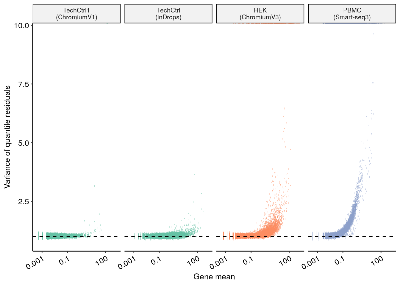
Distribution of means of poisson and non-poisson genes
plot.kde <- PlotKDEPois(fits_df)
plot.kde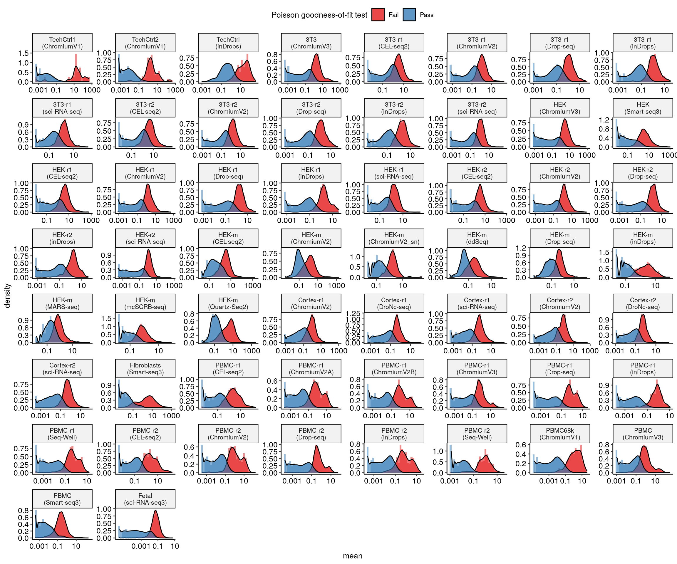
dir.create(here::here("output", "figures"), showWarnings = F, recursive = T)
ggsave(here::here("output", "figures", paste0("01_PoissonKDE_ncells_", ncells, "_residtype_", residual_type, ".pdf")), width = 12, height = 10)
Plot fraction of non-poisson
plot.poisvsumi <- PlotPoisVsUMI.cell_line(frac_df)
plot.poisvsumix <- plot.poisvsumi + theme(legend.position = c(0.5, 1.0))
plot.poisvsumix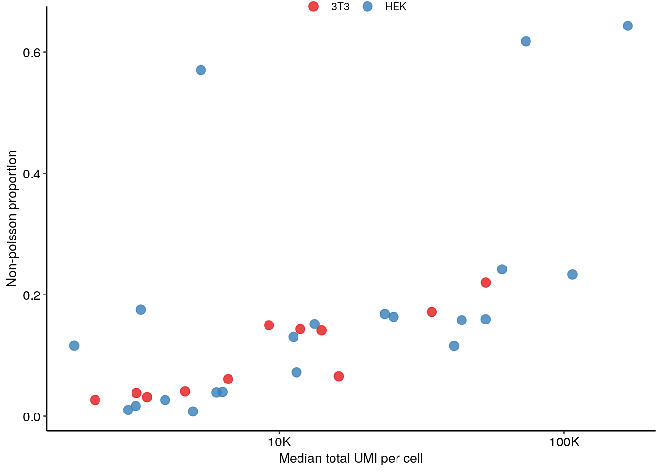
Downsampling
sample_name <- "PBMC__Smart-seq3"

root_dir <- here::here(paste0("output/snakemake_output/", sample_name, "_sampled_counts/poisson_glm_output/", ncells))


downsampled_umis <- c(
  10000, 7500, 5000,
  2000, 1000
)


names(downsampled_umis)<- c(
  "10,000", "7,500", "5,000",
  "2,000", "1,000"
)

sampled_dataset_keys <- paste0(sample_name, "_sampled_", downsampled_umis)

sampled_counts <- list()

for (name in downsampled_umis) {
  seu <- readRDS(here::here("data", "sampled_counts", paste0(sample_name, "_sampled_counts"), paste0(sample_name, "_sampled_", name, ".rds")))
  sampled_counts[[as.character(name)]] <- GetAssayData(seu, assay = "RNA", slot = "counts")
}

sampled <- readRDS(here::here("data", "rds_filtered", paste0(sample_name, ".rds")))
counts <- GetAssayData(sampled, assay = "RNA", slot = "counts")
counts_totalumis <- colSums2(counts)

generated_poissons <- list()

PredictPoisson <- function(counts_df) {
  predicted_poisson <- dpois(counts_df$counts, lambda = mean(counts_df$counts))
  return(predicted_poisson)
}

goi <- c("RPS19", "TPT1")
names(goi) <- goi

PredictPoisson <- function(counts_df) {
  predicted_poisson <- dpois(counts_df$counts, lambda = mean(counts_df$counts))
  return(predicted_poisson)
}

med_libsize <- "8,288" #(median(colSums2(counts)))

for (gene_name in names(goi)) {
  gene <- goi[[gene_name]]
  c1 <- "5000"
  c2 <- "1000"
  counts_goi_full <- counts[gene, ]
  counts_goi_full_subset <- counts_goi_full[counts_goi_full > 1]
  counts_goi_5k <- sampled_counts[[c1]][gene, ]
  counts_goi_1k <- sampled_counts[[c2]][gene, ]

  counts_df_full <- data.frame(counts = counts_goi_full_subset)
  counts_df_5k <- data.frame(counts = counts_goi_5k)
  counts_df_1k <- data.frame(counts = counts_goi_1k)

  labels <- c(
    paste0("Original  ", med_libsize, " UMI/cell"),
    paste0("Sampled ", so_formatter(as.integer(c1)), " UMI/cell"),
    paste0("Sampled ", so_formatter(as.integer(c2)), " UMI/cell")
  )
  counts_df_full$predicted_poisson <- PredictPoisson(counts_df_full)
  counts_df_full$sampletype <- labels[1]
  counts_df_5k$predicted_poisson <- PredictPoisson(counts_df_5k)
  counts_df_5k$sampletype <- labels[2]
  counts_df_1k$predicted_poisson <- PredictPoisson(counts_df_1k)
  counts_df_1k$sampletype <- labels[3]

  merged_counts <- rbind(counts_df_full, counts_df_5k, counts_df_1k)
  merged_counts$sampletype <- factor(merged_counts$sampletype, levels = labels)
  generated_poissons[[gene_name]] <- merged_counts
}
generated_poissons_df <- bind_rows(generated_poissons, .id = "gene")


plot.genespois <- ggplot(generated_poissons_df, aes(x = counts)) +
  geom_histogram(aes(y = ..density..), binwidth = 1, colour = "gray", fill = "white") +
  geom_line(aes(counts, predicted_poisson), color = "red") +
  facet_wrap(gene ~ sampletype, scales = "free", ncol = 3) +
  xlab("Counts") +
  ylab("Density") +
  scale_y_continuous(breaks = c(0.00, 0.10, 0.20))
plot.genespois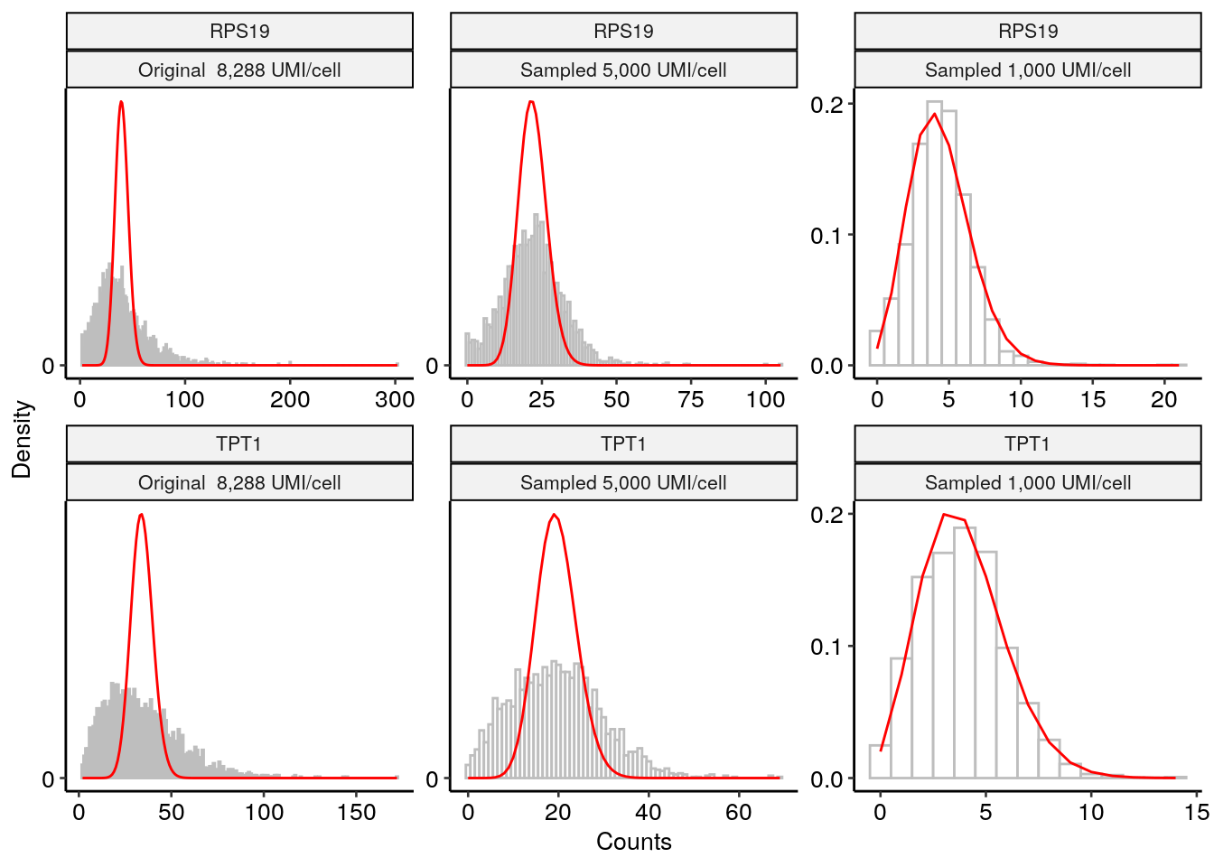
ncells <- "1000"
residual_type <- "quantile"
nb_column <- paste0("qval_ssr", "_", residual_type)
ssr_column <- paste0("ssr", "_", residual_type, "_normalized")


results_df <- GetFits.sampled(root_dir, nb_column)
fits_df.sampledx <- results_df$fits
frac_df.sampled <- results_df$frac_df

fits_df.sampled <- ProcessFits.sampled(fits_df.sampledx, nb_column)
fits_df.sampled$umi <- stringr::str_split_fixed(fits_df.sampled$key, pattern = "_", n = 5)[, 5]
frac_df.sampled$umi <- stringr::str_split_fixed(frac_df.sampled$key, pattern = "_", n = 5)[, 5]

fits_df.sampled$umi <- factor(fits_df.sampled$umi, levels = as.character(downsampled_umis), labels = paste0("Sampled ", names(downsampled_umis), " UMI/cell"))

frac_df.sampled$umi <- factor(frac_df.sampled$umi, levels = as.character(downsampled_umis), labels = paste0("Sampled ", names(downsampled_umis), " UMI/cell"))
fits_df.sampled$sample_name <- fits_df.sampled$umi
fits_df.sampled$datatype <- "heterogeneous"
fits_df.sampled$datatype <- factor(fits_df.sampled$datatype, levels = c("technical-control", "cell line", "heterogeneous"))
fits_df.sampled.subset <- fits_df.sampled[!is.na(fits_df.sampled[, ssr_column]), ]
plot.glmresiddownsample <- PlotGLMResiduals.sampled(fits_df.sampled, y = ssr_column, ncol = 5) + ylab(paste0("Variance of ", residual_type, " residuals"))
plot.glmresiddownsample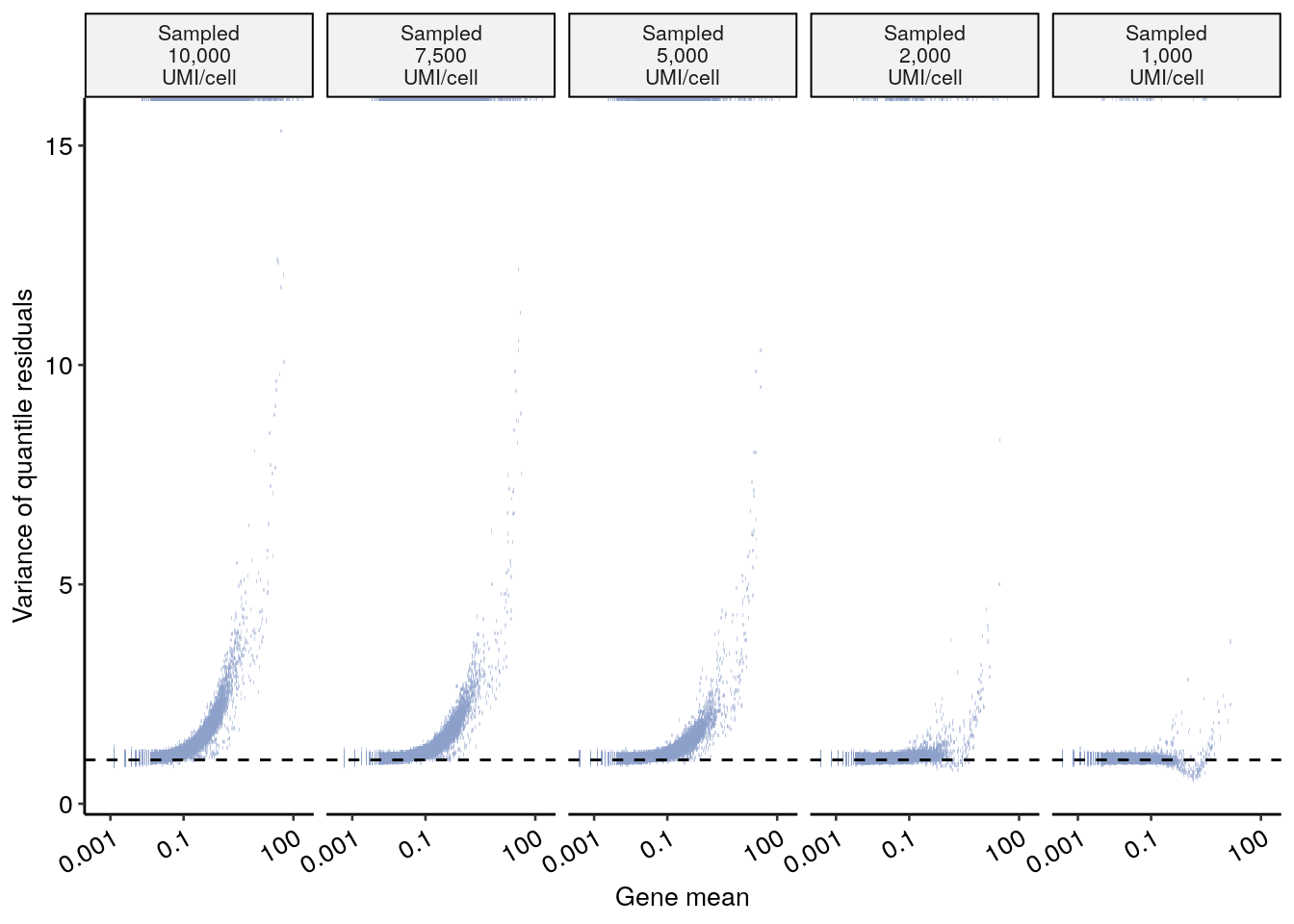
frac_df.sampled.subset <- frac_df.sampled[, c(
  "umi", "median_cell_total_umi", "median_gene_total_umi",
  "median_gene_avg_umi", "nonpoisson_fraction"
)]

kbl(frac_df.sampled.subset, booktabs = T) %>%
kable_styling(latex_options = "striped")| umi | median_cell_total_umi | median_gene_total_umi | median_gene_avg_umi | nonpoisson_fraction |
|---|---|---|---|---|
| Sampled 10,000 UMI/cell | 9998 | 29 | 0.0366162 | 0.4677393 |
| Sampled 7,500 UMI/cell | 7500 | 28 | 0.0280000 | 0.3953927 |
| Sampled 5,000 UMI/cell | 5000 | 23 | 0.0230000 | 0.2820475 |
| Sampled 2,000 UMI/cell | 2000 | 14 | 0.0140000 | 0.0219026 |
| Sampled 1,000 UMI/cell | 999 | 11 | 0.0110000 | 0.0049998 |
print(xtable(frac_df.sampled.subset, type = "latex", digits=3), include.rownames = FALSE, file=here::here("output", "tables", "frac_nonpoisson_sampled.tex"))plot.poisvsumi <- PlotPoisVsUMI.cell_line(frac_df) + # theme(legend.position = "top")
theme(legend.position = c(0.5, 1.04))
layout <- "
AAAA
BBBC
DDDD
EEEE
"
plot.dots +
plot.glmresid4 + plot.poisvsumi +
plot.genespois + plot.glmresiddownsample +
plot_layout(design = layout, tag_level = "new") + plot_annotation(tag_levels = "A") & theme(plot.tag = element_text(face = "bold"))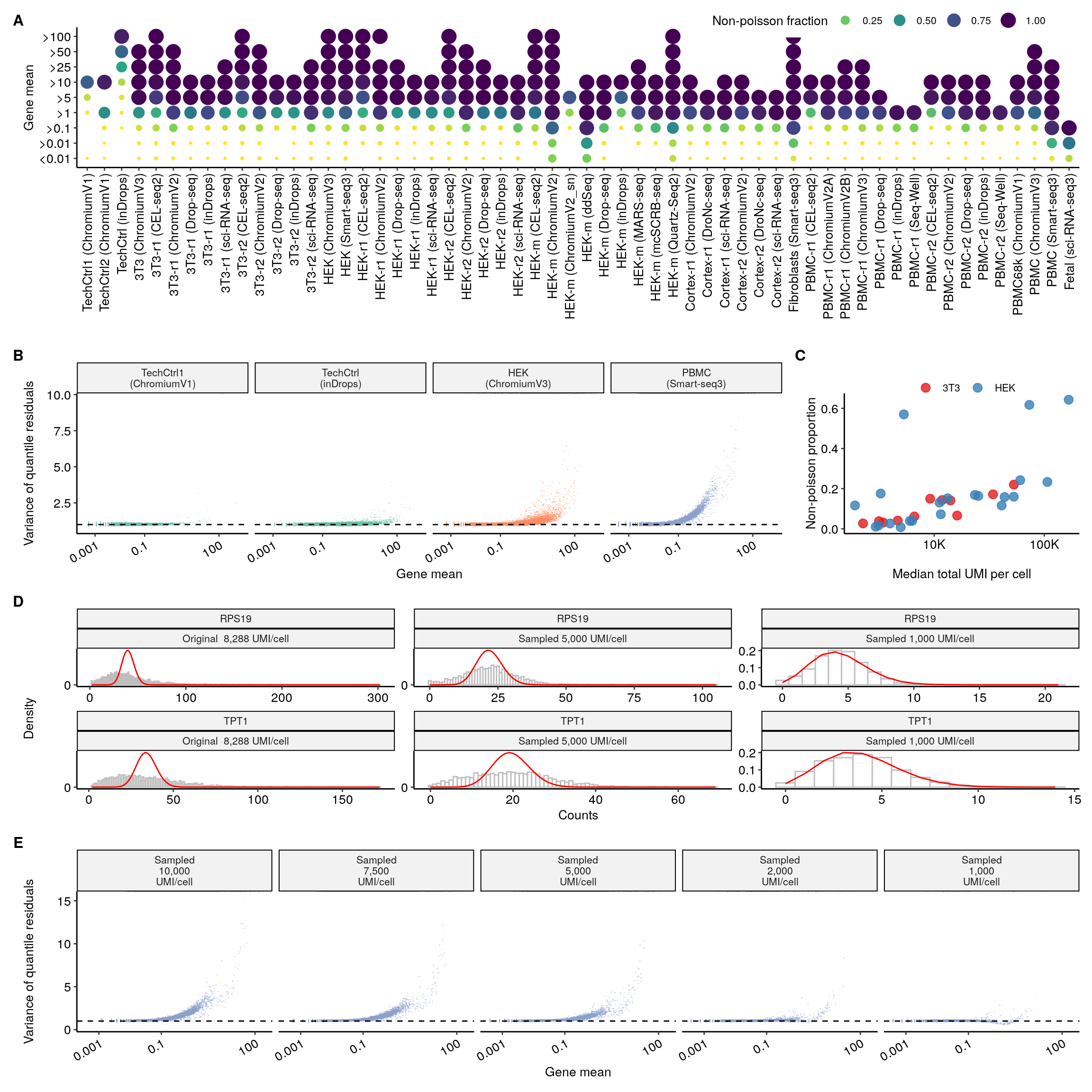
ggsave(here::here("output", "figures", "01_Figure1.pdf"), width = 12, height = 15)sessionInfo()R version 4.0.0 (2020-04-24)
Platform: x86_64-pc-linux-gnu (64-bit)
Running under: Ubuntu 18.04.5 LTS
Matrix products: default
BLAS: /usr/lib/x86_64-linux-gnu/blas/libblas.so.3.7.1
LAPACK: /usr/lib/x86_64-linux-gnu/lapack/liblapack.so.3.7.1
locale:
[1] LC_CTYPE=en_US.UTF-8 LC_NUMERIC=C
[3] LC_TIME=en_US.UTF-8 LC_COLLATE=en_US.UTF-8
[5] LC_MONETARY=en_US.UTF-8 LC_MESSAGES=en_US.UTF-8
[7] LC_PAPER=en_US.UTF-8 LC_NAME=C
[9] LC_ADDRESS=C LC_TELEPHONE=C
[11] LC_MEASUREMENT=en_US.UTF-8 LC_IDENTIFICATION=C
attached base packages:
[1] stats graphics grDevices utils datasets methods base
other attached packages:
[1] xtable_1.8-4 sparseMatrixStats_1.2.1 MatrixGenerics_1.2.1
[4] matrixStats_0.59.0 SeuratObject_4.0.2 Seurat_4.0.3
[7] scattermore_0.7 reshape2_1.4.4 readr_1.4.0
[10] RColorBrewer_1.1-2 patchwork_1.1.1 kableExtra_1.3.4
[13] here_1.0.1 ggridges_0.5.3 ggpubr_0.4.0
[16] ggplot2_3.3.5 dplyr_1.0.7 workflowr_1.6.2
loaded via a namespace (and not attached):
[1] readxl_1.3.1 backports_1.2.1 systemfonts_1.0.2
[4] plyr_1.8.6 igraph_1.2.6 lazyeval_0.2.2
[7] splines_4.0.0 listenv_0.8.0 digest_0.6.27
[10] htmltools_0.5.1.1 fansi_0.5.0 magrittr_2.0.1
[13] tensor_1.5 cluster_2.1.0 ROCR_1.0-11
[16] openxlsx_4.2.4 globals_0.14.0 svglite_2.0.0
[19] spatstat.sparse_2.0-0 colorspace_2.0-2 rvest_1.0.0
[22] ggrepel_0.9.1 textshaping_0.3.5 haven_2.4.1
[25] xfun_0.24 crayon_1.4.1 jsonlite_1.7.2
[28] spatstat.data_2.1-0 survival_3.2-7 zoo_1.8-9
[31] glue_1.4.2 polyclip_1.10-0 gtable_0.3.0
[34] webshot_0.5.2 leiden_0.3.8 car_3.0-10
[37] future.apply_1.7.0 abind_1.4-5 scales_1.1.1
[40] DBI_1.1.1 rstatix_0.7.0 miniUI_0.1.1.1
[43] Rcpp_1.0.6 viridisLite_0.4.0 reticulate_1.20
[46] spatstat.core_2.2-0 foreign_0.8-79 htmlwidgets_1.5.3
[49] httr_1.4.2 ellipsis_0.3.2 ica_1.0-2
[52] farver_2.1.0 pkgconfig_2.0.3 uwot_0.1.10
[55] sass_0.4.0 deldir_0.2-10 utf8_1.2.1
[58] labeling_0.4.2 tidyselect_1.1.1 rlang_0.4.11
[61] later_1.2.0 munsell_0.5.0 cellranger_1.1.0
[64] tools_4.0.0 generics_0.1.0 broom_0.7.8
[67] evaluate_0.14 stringr_1.4.0 fastmap_1.1.0
[70] ragg_1.1.3 yaml_2.2.1 goftest_1.2-2
[73] knitr_1.33 fs_1.5.0 fitdistrplus_1.1-5
[76] zip_2.2.0 purrr_0.3.4 RANN_2.6.1
[79] pbapply_1.4-3 future_1.21.0 nlme_3.1-152
[82] mime_0.11 xml2_1.3.2 compiler_4.0.0
[85] rstudioapi_0.13 plotly_4.9.4.1 curl_4.3.2
[88] png_0.1-7 ggsignif_0.6.2 spatstat.utils_2.2-0
[91] tibble_3.1.2 bslib_0.2.5.1 stringi_1.6.2
[94] highr_0.8 forcats_0.5.1 lattice_0.20-41
[97] Matrix_1.3-4 vctrs_0.3.8 pillar_1.6.1
[100] lifecycle_1.0.0 spatstat.geom_2.2-0 lmtest_0.9-38
[103] jquerylib_0.1.4 RcppAnnoy_0.0.18 data.table_1.14.0
[106] cowplot_1.1.1 irlba_2.3.3 httpuv_1.6.1
[109] R6_2.5.0 promises_1.2.0.1 KernSmooth_2.23-17
[112] gridExtra_2.3 rio_0.5.27 parallelly_1.26.0
[115] codetools_0.2-16 MASS_7.3-51.6 assertthat_0.2.1
[118] rprojroot_2.0.2 withr_2.4.2 sctransform_0.3.2.9008
[121] mgcv_1.8-33 parallel_4.0.0 hms_1.1.0
[124] rpart_4.1-15 grid_4.0.0 tidyr_1.1.3
[127] rmarkdown_2.9 carData_3.0-4 Rtsne_0.15
[130] git2r_0.26.1 shiny_1.6.0
sessionInfo()R version 4.0.0 (2020-04-24)
Platform: x86_64-pc-linux-gnu (64-bit)
Running under: Ubuntu 18.04.5 LTS
Matrix products: default
BLAS: /usr/lib/x86_64-linux-gnu/blas/libblas.so.3.7.1
LAPACK: /usr/lib/x86_64-linux-gnu/lapack/liblapack.so.3.7.1
locale:
[1] LC_CTYPE=en_US.UTF-8 LC_NUMERIC=C
[3] LC_TIME=en_US.UTF-8 LC_COLLATE=en_US.UTF-8
[5] LC_MONETARY=en_US.UTF-8 LC_MESSAGES=en_US.UTF-8
[7] LC_PAPER=en_US.UTF-8 LC_NAME=C
[9] LC_ADDRESS=C LC_TELEPHONE=C
[11] LC_MEASUREMENT=en_US.UTF-8 LC_IDENTIFICATION=C
attached base packages:
[1] stats graphics grDevices utils datasets methods base
other attached packages:
[1] xtable_1.8-4 sparseMatrixStats_1.2.1 MatrixGenerics_1.2.1
[4] matrixStats_0.59.0 SeuratObject_4.0.2 Seurat_4.0.3
[7] scattermore_0.7 reshape2_1.4.4 readr_1.4.0
[10] RColorBrewer_1.1-2 patchwork_1.1.1 kableExtra_1.3.4
[13] here_1.0.1 ggridges_0.5.3 ggpubr_0.4.0
[16] ggplot2_3.3.5 dplyr_1.0.7 workflowr_1.6.2
loaded via a namespace (and not attached):
[1] readxl_1.3.1 backports_1.2.1 systemfonts_1.0.2
[4] plyr_1.8.6 igraph_1.2.6 lazyeval_0.2.2
[7] splines_4.0.0 listenv_0.8.0 digest_0.6.27
[10] htmltools_0.5.1.1 fansi_0.5.0 magrittr_2.0.1
[13] tensor_1.5 cluster_2.1.0 ROCR_1.0-11
[16] openxlsx_4.2.4 globals_0.14.0 svglite_2.0.0
[19] spatstat.sparse_2.0-0 colorspace_2.0-2 rvest_1.0.0
[22] ggrepel_0.9.1 textshaping_0.3.5 haven_2.4.1
[25] xfun_0.24 crayon_1.4.1 jsonlite_1.7.2
[28] spatstat.data_2.1-0 survival_3.2-7 zoo_1.8-9
[31] glue_1.4.2 polyclip_1.10-0 gtable_0.3.0
[34] webshot_0.5.2 leiden_0.3.8 car_3.0-10
[37] future.apply_1.7.0 abind_1.4-5 scales_1.1.1
[40] DBI_1.1.1 rstatix_0.7.0 miniUI_0.1.1.1
[43] Rcpp_1.0.6 viridisLite_0.4.0 reticulate_1.20
[46] spatstat.core_2.2-0 foreign_0.8-79 htmlwidgets_1.5.3
[49] httr_1.4.2 ellipsis_0.3.2 ica_1.0-2
[52] farver_2.1.0 pkgconfig_2.0.3 uwot_0.1.10
[55] sass_0.4.0 deldir_0.2-10 utf8_1.2.1
[58] labeling_0.4.2 tidyselect_1.1.1 rlang_0.4.11
[61] later_1.2.0 munsell_0.5.0 cellranger_1.1.0
[64] tools_4.0.0 generics_0.1.0 broom_0.7.8
[67] evaluate_0.14 stringr_1.4.0 fastmap_1.1.0
[70] ragg_1.1.3 yaml_2.2.1 goftest_1.2-2
[73] knitr_1.33 fs_1.5.0 fitdistrplus_1.1-5
[76] zip_2.2.0 purrr_0.3.4 RANN_2.6.1
[79] pbapply_1.4-3 future_1.21.0 nlme_3.1-152
[82] mime_0.11 xml2_1.3.2 compiler_4.0.0
[85] rstudioapi_0.13 plotly_4.9.4.1 curl_4.3.2
[88] png_0.1-7 ggsignif_0.6.2 spatstat.utils_2.2-0
[91] tibble_3.1.2 bslib_0.2.5.1 stringi_1.6.2
[94] highr_0.8 forcats_0.5.1 lattice_0.20-41
[97] Matrix_1.3-4 vctrs_0.3.8 pillar_1.6.1
[100] lifecycle_1.0.0 spatstat.geom_2.2-0 lmtest_0.9-38
[103] jquerylib_0.1.4 RcppAnnoy_0.0.18 data.table_1.14.0
[106] cowplot_1.1.1 irlba_2.3.3 httpuv_1.6.1
[109] R6_2.5.0 promises_1.2.0.1 KernSmooth_2.23-17
[112] gridExtra_2.3 rio_0.5.27 parallelly_1.26.0
[115] codetools_0.2-16 MASS_7.3-51.6 assertthat_0.2.1
[118] rprojroot_2.0.2 withr_2.4.2 sctransform_0.3.2.9008
[121] mgcv_1.8-33 parallel_4.0.0 hms_1.1.0
[124] rpart_4.1-15 grid_4.0.0 tidyr_1.1.3
[127] rmarkdown_2.9 carData_3.0-4 Rtsne_0.15
[130] git2r_0.26.1 shiny_1.6.0