Supplementary Figure 1
Last updated: 2021-07-06
Checks: 6 1
Knit directory: scRNA_NB_comparison/
This reproducible R Markdown analysis was created with workflowr (version 1.6.2). The Checks tab describes the reproducibility checks that were applied when the results were created. The Past versions tab lists the development history.
The R Markdown is untracked by Git. To know which version of the R Markdown file created these results, you’ll want to first commit it to the Git repo. If you’re still working on the analysis, you can ignore this warning. When you’re finished, you can run wflow_publish to commit the R Markdown file and build the HTML.
Great job! The global environment was empty. Objects defined in the global environment can affect the analysis in your R Markdown file in unknown ways. For reproduciblity it’s best to always run the code in an empty environment.
The command set.seed(20210706) was run prior to running the code in the R Markdown file. Setting a seed ensures that any results that rely on randomness, e.g. subsampling or permutations, are reproducible.
Great job! Recording the operating system, R version, and package versions is critical for reproducibility.
Nice! There were no cached chunks for this analysis, so you can be confident that you successfully produced the results during this run.
Great job! Using relative paths to the files within your workflowr project makes it easier to run your code on other machines.
Great! You are using Git for version control. Tracking code development and connecting the code version to the results is critical for reproducibility.
The results in this page were generated with repository version e0b7c2c. See the Past versions tab to see a history of the changes made to the R Markdown and HTML files.
Note that you need to be careful to ensure that all relevant files for the analysis have been committed to Git prior to generating the results (you can use wflow_publish or wflow_git_commit). workflowr only checks the R Markdown file, but you know if there are other scripts or data files that it depends on. Below is the status of the Git repository when the results were generated:
Ignored files:
    Ignored:    data/raw_data/
    Ignored:    data/rds_filtered/
    Ignored:    data/rds_raw/
    Ignored:    output/snakemake_output/

Untracked files:
    Untracked:  analysis/01_Smart-seq3.Rmd
    Untracked:  analysis/02_Mereu.Rmd
    Untracked:  analysis/03A_Ding-Mixture-HEK-3T3.Rmd
    Untracked:  analysis/03B_Ding-PBMC.Rmd
    Untracked:  analysis/03C_Ding-Cortex.Rmd
    Untracked:  analysis/04_PBMC68k.Rmd
    Untracked:  analysis/05_Fetal-sciRNAseq3.Rmd
    Untracked:  analysis/06G_VS2020_Seurat.Rmd
    Untracked:  analysis/07_Filter_all_datasets.Rmd
    Untracked:  analysis/08_Downsample_PBMC__Smart-seq3.Rmd
    Untracked:  analysis/09_Figure1.Rmd
    Untracked:  analysis/10_Figure2.Rmd
    Untracked:  analysis/11_Figure3.Rmd
    Untracked:  analysis/12_SuppFigure-DataStats.Rmd
    Untracked:  analysis/13_SuppFigure-VST.Rmd
    Untracked:  analysis/14_SuppFigure-Simulation.Rmd
    Untracked:  analysis/15_SuppFigure-Upsampling.Rmd
    Untracked:  data/datasets.csv
    Untracked:  data/sampled_counts/
    Untracked:  output/figures/
    Untracked:  output/tables/

Unstaged changes:
    Modified:   .gitignore
    Modified:   analysis/_site.yml
    Modified:   analysis/about.Rmd
    Modified:   analysis/index.Rmd
    Modified:   analysis/license.Rmd
Note that any generated files, e.g. HTML, png, CSS, etc., are not included in this status report because it is ok for generated content to have uncommitted changes.
There are no past versions. Publish this analysis with wflow_publish() to start tracking its development.
suppressPackageStartupMessages({
  library(dplyr)
  library(ggplot2)
  library(kableExtra)
  library(ggpubr)
  library(ggridges)
  library(here)
  library(patchwork)
  library(RColorBrewer)
  library(readr)
  library(reshape2)
  library(scattermore)
  library(Seurat)
  library(sparseMatrixStats)
  library(xtable)
})
`%notin%` <- Negate(`%in%`)
theme_set(theme_pubr(base_size = 9))
knitr::opts_chunk$set(warning = FALSE, message = FALSE)


clean_keys <- function(key) {
  gsub(
    pattern = "|\\)", replacement = "",
    x = gsub(pattern = " |\\(", replacement = "_", x = key)
  )
}
CellSummary <- function(cm) {
total_umi_per_cell <- colSums(cm)
expressed_features_per_cell <- colSums(x = cm > 0)
n_features <- dim(cm)[1]
nonexpressed_features_per_cell <- n_features - expressed_features_per_cell
median_umi_per_cell <- median(total_umi_per_cell)
avg_umi_per_cell <- total_umi_per_cell / n_features
avg_umi_per_cell_expressedgenes <- total_umi_per_cell / expressed_features_per_cell
cell_amean <- colMeans2(cm)
cell_variance <- colVars(cm)
cell_attr <- data.frame(
total_umi = total_umi_per_cell, n_expressed_genes = expressed_features_per_cell, n_nonexpressed_cells = nonexpressed_features_per_cell, prop_expressed_genes = expressed_features_per_cell / n_features,
prop_nonexpressed_genes = nonexpressed_features_per_cell / n_features,
avg_umi = avg_umi_per_cell, avg_umi_expressedgenes = avg_umi_per_cell_expressedgenes, cell_amean = cell_amean,
cell_variance = cell_variance
)
return(cell_attr)
}
GeneSummary <- function(cm) {
# remove genes and cells with zero counts
cm <- cm[rowSums(cm) > 0, colSums(cm) > 0]
total_umi_per_gene <- rowSums(cm)
expressed_cells_per_gene <- rowSums(cm > 0)
n_cells <- dim(cm)[2]
nonexpressed_cells_per_gene <- n_cells - expressed_cells_per_gene
median_umi_per_gene <- median(total_umi_per_gene)
avg_umi_per_gene <- total_umi_per_gene / n_cells
avg_umi_per_gene_expressedcells <- total_umi_per_gene / expressed_cells_per_gene
gene_amean <- rowMeans(cm)
gene_var <- rowVars(cm)
gene_gmean <- sctransform:::row_gmean(cm)
gene_attr <- data.frame(
total_umi = total_umi_per_gene, n_expressed_cells = expressed_cells_per_gene, n_nonexpressed_cells = nonexpressed_cells_per_gene, prop_expressed_cells = expressed_cells_per_gene / n_cells,
prop_nonexpressed_cells = nonexpressed_cells_per_gene / n_cells,
avg_umi = avg_umi_per_gene, avg_umi_expressedcells = avg_umi_per_gene_expressedcells, gene_amean = gene_amean, gene_gmean = gene_gmean, gene_variance = gene_var
)
return(gene_attr)
}
GetGeneCellSummary <- function(dataset_name, mode = "gene") {
cm <- GetAssayData(
readRDS(here::here("data", "rds_filtered", paste0(clean_keys(dataset_name), ".rds"))),
assay = "RNA", slot = "counts"
)
if (mode == "gene") {
gc_attr <- GeneSummary(cm)
} else {
gc_attr <- CellSummary(cm)
}
cm <- NULL
gc()
return(gc_attr)
}datasets <- readr::read_csv(here::here("data", "datasets.csv"), col_types = readr::cols())
dataset_keys <- datasets$key
counts <- sapply(dataset_keys,
FUN = function(x) {
GetAssayData(
readRDS(here::here("data", "rds_filtered", paste0(clean_keys(x), ".rds"))),
assay = "RNA", slot = "counts"
)
},
simplify = FALSE, USE.NAMES = TRUE
)
cell_attrs <- sapply(dataset_keys,
FUN = function(x) {
message(x)
GetGeneCellSummary(x, "cell")
},
simplify = FALSE, USE.NAMES = TRUE
)
cell_attrs_df <- bind_rows(cell_attrs, .id = "key")
cell_attrs_df <- left_join(cell_attrs_df, datasets)
gene_attrs <- sapply(dataset_keys,
FUN = function(x) {
GetGeneCellSummary(x, "gene")
},
simplify = FALSE, USE.NAMES = TRUE
)
gene_attrs_df <- bind_rows(gene_attrs, .id = "key")
gene_attrs_df <- left_join(gene_attrs_df, datasets)UMI statistics
gene_attrs_df$datatype <- factor(gene_attrs_df$datatype, levels = c("technical-control", "cell line", "heterogeneous"))
cell_attrs_df$datatype <- factor(cell_attrs_df$datatype, levels = c("technical-control", "cell line", "heterogeneous"))

gene_attrs_df_summary <- gene_attrs_df %>%
  group_by(sample_name) %>%
  summarize(median.zero_prop = round(median(prop_nonexpressed_cells), 4), median.detection_rate = round(median(prop_expressed_cells), 4))

gene_attrs_df_summary <- left_join(gene_attrs_df_summary, datasets)

pgeneavg <- ggplot(gene_attrs_df, aes(
  x = avg_umi,
  y = reorder(sample_name, avg_umi, FUN = median),
  avg_umi, fill = datatype
)) +
  # scale_x_log10() +
  scale_x_continuous(trans = "log10", breaks = c(0.0001, 0.01, 1, 100, 10000), labels = c("0.0001", 0.01, 1, 100, 10000)) +
  stat_density_ridges(quantile_lines = TRUE, quantiles = 2) +
  scale_fill_manual(values = brewer.pal(3, "Set2"), name = "") +
  labs(title = "") +
  ylab("") +
  theme(
    legend.position = "bottom",
    legend.direction = "horizontal",
    legend.background = element_blank()
  ) +
  guides(col = guide_legend(ncol = 3)) +
  xlab("Mean UMI per gene")


cell_attrs_df_summary <- cell_attrs_df %>%
  group_by(sample_name, datatype) %>%
  summarize(median_umi = median(total_umi), median_detection_rate = round(median(prop_expressed_genes), 3))
# cell_attrs_df_summary
pcelltot <- ggplot(cell_attrs_df, aes(
  x = total_umi,
  y = reorder(sample_name, total_umi, FUN = median),
  total_umi, fill = datatype
)) +
  scale_x_continuous(trans = "log10", breaks = c(0.0001, 0.01, 0.1, 1, 10, 100, 1000, 10000, 100000), labels = c("0.0001", 0.01, 0.1, 1, 10, 100, 1000, 10000, "100000")) +
  stat_density_ridges(quantile_lines = TRUE, quantiles = 2) +
  scale_fill_manual(values = brewer.pal(3, "Set2"), name = "") +
  labs(title = "") +
  ylab("") +
  theme(
    legend.position = "bottom",
    legend.direction = "horizontal",
    legend.background = element_blank()
  ) +
  guides(col = guide_legend(ncol = 3)) +
  xlab("Total UMI per cell")

wrap_plots(pcelltot,pgeneavg, ncol = 2) + plot_annotation(tag_levels = "A") + plot_layout(guides = "collect", tag_level = "new") & theme(legend.position = "bottom") & theme(plot.tag = element_text(face = "bold"))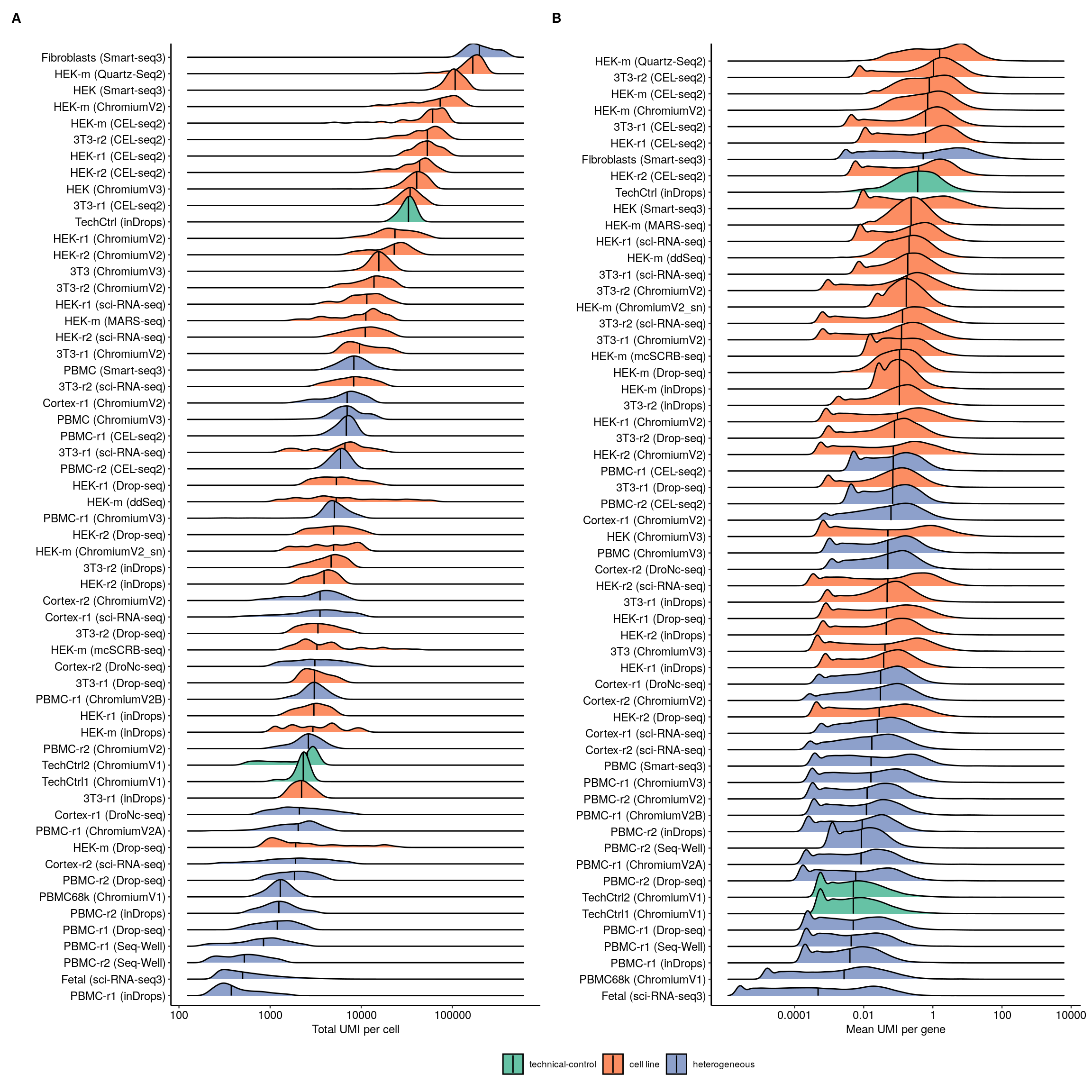
dir.create(here::here("output", "figures"), showWarnings = F)

ggsave(here::here("output", "figures", "data_stats.pdf"), width = 12, height = 12, dpi = "print")
cell_attrs_df_summary <- cell_attrs_df_summary %>% arrange(median_umi)
kbl(cell_attrs_df_summary, booktabs = T) %>%
kable_styling(latex_options = "striped")| sample_name | datatype | median_umi | median_detection_rate |
|---|---|---|---|
| PBMC-r1 (inDrops) | heterogeneous | 375.0 | 0.009 |
| Fetal (sci-RNA-seq3) | heterogeneous | 499.0 | 0.008 |
| PBMC-r2 (Seq-Well) | heterogeneous | 521.0 | 0.011 |
| PBMC-r1 (Seq-Well) | heterogeneous | 846.0 | 0.017 |
| PBMC-r1 (Drop-seq) | heterogeneous | 1199.0 | 0.022 |
| PBMC-r2 (inDrops) | heterogeneous | 1247.0 | 0.020 |
| PBMC68k (ChromiumV1) | heterogeneous | 1292.0 | 0.026 |
| PBMC-r2 (Drop-seq) | heterogeneous | 1850.5 | 0.030 |
| Cortex-r2 (sci-RNA-seq) | heterogeneous | 1899.0 | 0.044 |
| HEK-m (Drop-seq) | cell line | 1907.5 | 0.051 |
| PBMC-r1 (ChromiumV2A) | heterogeneous | 2032.0 | 0.027 |
| Cortex-r1 (DroNc-seq) | heterogeneous | 2092.0 | 0.053 |
| 3T3-r1 (inDrops) | cell line | 2213.0 | 0.061 |
| TechCtrl1 (ChromiumV1) | technical-control | 2308.5 | 0.031 |
| TechCtrl2 (ChromiumV1) | technical-control | 2566.0 | 0.031 |
| PBMC-r2 (ChromiumV2) | heterogeneous | 2626.0 | 0.036 |
| HEK-m (inDrops) | cell line | 2943.0 | 0.073 |
| HEK-r1 (inDrops) | cell line | 3019.0 | 0.057 |
| PBMC-r1 (ChromiumV2B) | heterogeneous | 3050.0 | 0.037 |
| 3T3-r1 (Drop-seq) | cell line | 3072.0 | 0.082 |
| Cortex-r2 (DroNc-seq) | heterogeneous | 3094.0 | 0.071 |
| HEK-m (mcSCRB-seq) | cell line | 3266.5 | 0.063 |
| 3T3-r2 (Drop-seq) | cell line | 3345.0 | 0.091 |
| Cortex-r1 (sci-RNA-seq) | heterogeneous | 3524.0 | 0.060 |
| Cortex-r2 (ChromiumV2) | heterogeneous | 3527.0 | 0.073 |
| HEK-r2 (inDrops) | cell line | 3904.0 | 0.073 |
| 3T3-r2 (inDrops) | cell line | 4666.5 | 0.107 |
| HEK-m (ChromiumV2_sn) | cell line | 4967.0 | 0.128 |
| HEK-r2 (Drop-seq) | cell line | 4968.5 | 0.085 |
| PBMC-r1 (ChromiumV3) | heterogeneous | 5066.0 | 0.054 |
| HEK-m (ddSeq) | cell line | 5304.5 | 0.108 |
| HEK-r1 (Drop-seq) | cell line | 5328.0 | 0.092 |
| PBMC-r2 (CEL-seq2) | heterogeneous | 5917.0 | 0.087 |
| 3T3-r1 (sci-RNA-seq) | cell line | 6609.5 | 0.136 |
| PBMC-r1 (CEL-seq2) | heterogeneous | 6848.0 | 0.096 |
| PBMC (ChromiumV3) | heterogeneous | 6992.0 | 0.107 |
| Cortex-r1 (ChromiumV2) | heterogeneous | 6993.5 | 0.122 |
| 3T3-r2 (sci-RNA-seq) | cell line | 8256.0 | 0.160 |
| PBMC (Smart-seq3) | heterogeneous | 8288.0 | 0.058 |
| 3T3-r1 (ChromiumV2) | cell line | 9548.0 | 0.140 |
| HEK-r2 (sci-RNA-seq) | cell line | 11045.0 | 0.160 |
| HEK-m (MARS-seq) | cell line | 11207.5 | 0.180 |
| HEK-r1 (sci-RNA-seq) | cell line | 11490.0 | 0.158 |
| 3T3-r2 (ChromiumV2) | cell line | 13776.5 | 0.185 |
| 3T3 (ChromiumV3) | cell line | 15577.0 | 0.180 |
| HEK-r2 (ChromiumV2) | cell line | 22986.5 | 0.171 |
| HEK-r1 (ChromiumV2) | cell line | 23388.0 | 0.169 |
| TechCtrl (inDrops) | technical-control | 32905.0 | 0.391 |
| 3T3-r1 (CEL-seq2) | cell line | 34291.0 | 0.321 |
| HEK (ChromiumV3) | cell line | 40547.0 | 0.246 |
| HEK-r2 (CEL-seq2) | cell line | 43670.0 | 0.287 |
| HEK-r1 (CEL-seq2) | cell line | 52973.0 | 0.308 |
| 3T3-r2 (CEL-seq2) | cell line | 53036.0 | 0.367 |
| HEK-m (CEL-seq2) | cell line | 60592.5 | 0.479 |
| HEK-m (ChromiumV2) | cell line | 73333.5 | 0.434 |
| HEK (Smart-seq3) | cell line | 106996.0 | 0.381 |
| HEK-m (Quartz-Seq2) | cell line | 167199.0 | 0.548 |
| Fibroblasts (Smart-seq3) | heterogeneous | 197151.0 | 0.380 |
dir.create(here::here("output", "tables"), showWarnings = F)
print(xtable(cell_attrs_df_summary, type = "latex", digits=3), include.rownames = FALSE, file = here::here("output", "tables", "datasets_umi_stats.tex"))
sessionInfo()R version 4.0.0 (2020-04-24)
Platform: x86_64-pc-linux-gnu (64-bit)
Running under: Ubuntu 18.04.5 LTS
Matrix products: default
BLAS: /usr/lib/x86_64-linux-gnu/blas/libblas.so.3.7.1
LAPACK: /usr/lib/x86_64-linux-gnu/lapack/liblapack.so.3.7.1
locale:
[1] LC_CTYPE=en_US.UTF-8 LC_NUMERIC=C
[3] LC_TIME=en_US.UTF-8 LC_COLLATE=en_US.UTF-8
[5] LC_MONETARY=en_US.UTF-8 LC_MESSAGES=en_US.UTF-8
[7] LC_PAPER=en_US.UTF-8 LC_NAME=C
[9] LC_ADDRESS=C LC_TELEPHONE=C
[11] LC_MEASUREMENT=en_US.UTF-8 LC_IDENTIFICATION=C
attached base packages:
[1] stats graphics grDevices utils datasets methods base
other attached packages:
[1] xtable_1.8-4 sparseMatrixStats_1.2.1 MatrixGenerics_1.2.1
[4] matrixStats_0.59.0 SeuratObject_4.0.2 Seurat_4.0.3
[7] scattermore_0.7 reshape2_1.4.4 readr_1.4.0
[10] RColorBrewer_1.1-2 patchwork_1.1.1 here_1.0.1
[13] ggridges_0.5.3 ggpubr_0.4.0 kableExtra_1.3.4
[16] ggplot2_3.3.5 dplyr_1.0.7 workflowr_1.6.2
loaded via a namespace (and not attached):
[1] readxl_1.3.1 backports_1.2.1 systemfonts_1.0.2
[4] plyr_1.8.6 igraph_1.2.6 lazyeval_0.2.2
[7] splines_4.0.0 listenv_0.8.0 digest_0.6.27
[10] htmltools_0.5.1.1 fansi_0.5.0 magrittr_2.0.1
[13] tensor_1.5 cluster_2.1.0 ROCR_1.0-11
[16] openxlsx_4.2.4 globals_0.14.0 svglite_2.0.0
[19] spatstat.sparse_2.0-0 colorspace_2.0-2 rvest_1.0.0
[22] ggrepel_0.9.1 textshaping_0.3.5 haven_2.4.1
[25] xfun_0.24 crayon_1.4.1 jsonlite_1.7.2
[28] spatstat.data_2.1-0 survival_3.2-7 zoo_1.8-9
[31] glue_1.4.2 polyclip_1.10-0 gtable_0.3.0
[34] webshot_0.5.2 leiden_0.3.8 car_3.0-10
[37] future.apply_1.7.0 abind_1.4-5 scales_1.1.1
[40] DBI_1.1.1 rstatix_0.7.0 miniUI_0.1.1.1
[43] Rcpp_1.0.6 viridisLite_0.4.0 reticulate_1.20
[46] spatstat.core_2.2-0 foreign_0.8-79 htmlwidgets_1.5.3
[49] httr_1.4.2 ellipsis_0.3.2 ica_1.0-2
[52] farver_2.1.0 pkgconfig_2.0.3 uwot_0.1.10
[55] sass_0.4.0 deldir_0.2-10 utf8_1.2.1
[58] tidyselect_1.1.1 rlang_0.4.11 later_1.2.0
[61] munsell_0.5.0 cellranger_1.1.0 tools_4.0.0
[64] generics_0.1.0 broom_0.7.8 evaluate_0.14
[67] stringr_1.4.0 fastmap_1.1.0 ragg_1.1.3
[70] yaml_2.2.1 goftest_1.2-2 knitr_1.33
[73] fs_1.5.0 fitdistrplus_1.1-5 zip_2.2.0
[76] purrr_0.3.4 RANN_2.6.1 pbapply_1.4-3
[79] future_1.21.0 nlme_3.1-152 mime_0.11
[82] xml2_1.3.2 compiler_4.0.0 rstudioapi_0.13
[85] plotly_4.9.4.1 curl_4.3.2 png_0.1-7
[88] ggsignif_0.6.2 spatstat.utils_2.2-0 tibble_3.1.2
[91] bslib_0.2.5.1 stringi_1.6.2 highr_0.8
[94] forcats_0.5.1 lattice_0.20-41 Matrix_1.3-4
[97] vctrs_0.3.8 pillar_1.6.1 lifecycle_1.0.0
[100] spatstat.geom_2.2-0 lmtest_0.9-38 jquerylib_0.1.4
[103] RcppAnnoy_0.0.18 data.table_1.14.0 cowplot_1.1.1
[106] irlba_2.3.3 httpuv_1.6.1 R6_2.5.0
[109] promises_1.2.0.1 KernSmooth_2.23-17 gridExtra_2.3
[112] rio_0.5.27 parallelly_1.26.0 codetools_0.2-16
[115] MASS_7.3-51.6 assertthat_0.2.1 rprojroot_2.0.2
[118] withr_2.4.2 sctransform_0.3.2.9008 mgcv_1.8-33
[121] parallel_4.0.0 hms_1.1.0 rpart_4.1-15
[124] grid_4.0.0 tidyr_1.1.3 rmarkdown_2.9
[127] carData_3.0-4 Rtsne_0.15 git2r_0.26.1
[130] shiny_1.6.0