Cardiac and TOP2 Genes - Log2CPM Boxplots
Last updated: 2025-02-18
Checks: 7 0
Knit directory: CX5461_Project/
This reproducible R Markdown analysis was created with workflowr (version 1.7.1). The Checks tab describes the reproducibility checks that were applied when the results were created. The Past versions tab lists the development history.
Great! Since the R Markdown file has been committed to the Git repository, you know the exact version of the code that produced these results.
Great job! The global environment was empty. Objects defined in the global environment can affect the analysis in your R Markdown file in unknown ways. For reproduciblity it’s best to always run the code in an empty environment.
The command set.seed(20250129) was run prior to running
the code in the R Markdown file. Setting a seed ensures that any results
that rely on randomness, e.g. subsampling or permutations, are
reproducible.
Great job! Recording the operating system, R version, and package versions is critical for reproducibility.
Nice! There were no cached chunks for this analysis, so you can be confident that you successfully produced the results during this run.
Great job! Using relative paths to the files within your workflowr project makes it easier to run your code on other machines.
Great! You are using Git for version control. Tracking code development and connecting the code version to the results is critical for reproducibility.
The results in this page were generated with repository version 55dbfa0. See the Past versions tab to see a history of the changes made to the R Markdown and HTML files.
Note that you need to be careful to ensure that all relevant files for
the analysis have been committed to Git prior to generating the results
(you can use wflow_publish or
wflow_git_commit). workflowr only checks the R Markdown
file, but you know if there are other scripts or data files that it
depends on. Below is the status of the Git repository when the results
were generated:
Ignored files:
    Ignored:    .RData
    Ignored:    .Rhistory
    Ignored:    .Rproj.user/

Staged changes:
    New:        data/DNA_Damage.csv
Note that any generated files, e.g. HTML, png, CSS, etc., are not included in this status report because it is ok for generated content to have uncommitted changes.
These are the previous versions of the repository in which changes were
made to the R Markdown
(analysis/Cardiac_and_TOP2_Genes.Rmd) and HTML
(docs/Cardiac_and_TOP2_Genes.html) files. If you’ve
configured a remote Git repository (see ?wflow_git_remote),
click on the hyperlinks in the table below to view the files as they
were in that past version.
| File | Version | Author | Date | Message |
|---|---|---|---|---|
| html | 55dbfa0 | sayanpaul01 | 2025-02-18 | Build site. |
| Rmd | 1b220ad | sayanpaul01 | 2025-02-18 | Updated analysis of Cardiac, TOP2, and DNA Damage Genes |
| html | 0a7f53e | sayanpaul01 | 2025-02-18 | Build site. |
| Rmd | 565ede2 | sayanpaul01 | 2025-02-18 | Updated analysis of Cardiac, TOP2, and DNA Damage Genes |
| html | 3313173 | sayanpaul01 | 2025-02-18 | Build site. |
| html | 456790a | sayanpaul01 | 2025-02-18 | Build site. |
| Rmd | e943e2d | sayanpaul01 | 2025-02-18 | Added TP53 as a DNA damage marker in log2CPM boxplots |
| html | 6ed78e2 | sayanpaul01 | 2025-02-09 | Build site. |
| html | 72599ac | sayanpaul01 | 2025-02-09 | Build site. |
| Rmd | 0e79f5b | sayanpaul01 | 2025-02-09 | Fix Timepoint Ordering in Boxplots |
| html | a41bd50 | sayanpaul01 | 2025-02-09 | Build site. |
| Rmd | 91f5f8f | sayanpaul01 | 2025-02-09 | Fix Timepoint Ordering in Boxplots |
| html | bcc58f6 | sayanpaul01 | 2025-02-09 | Build site. |
| html | 8c1912f | sayanpaul01 | 2025-02-09 | Build site. |
| Rmd | c6b5ccd | sayanpaul01 | 2025-02-09 | Fixed boxplot significance issue for Cardiac and TOP2 genes |
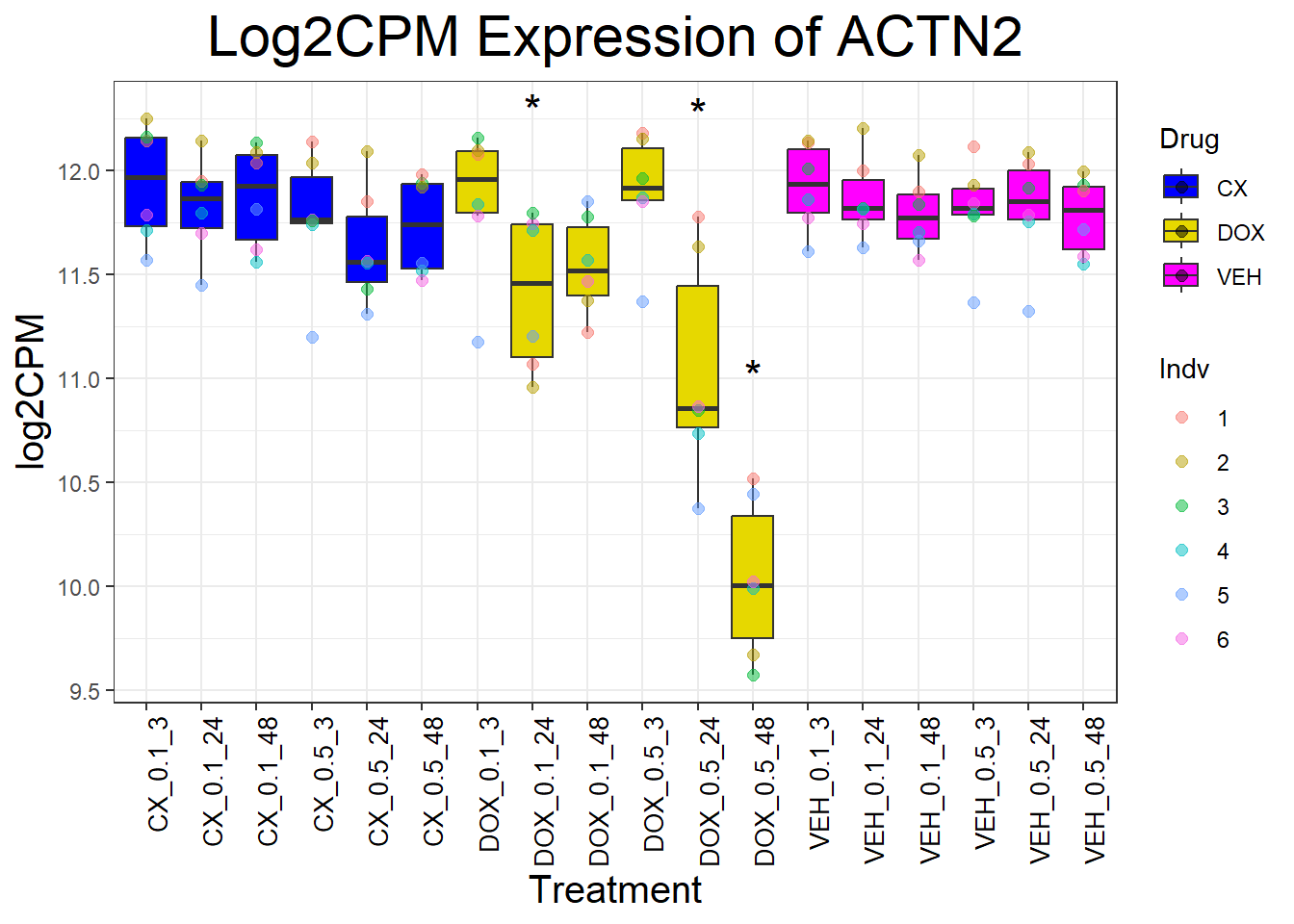
📌 Log2CPM Boxplots for Cardiac and TOP2 Genes
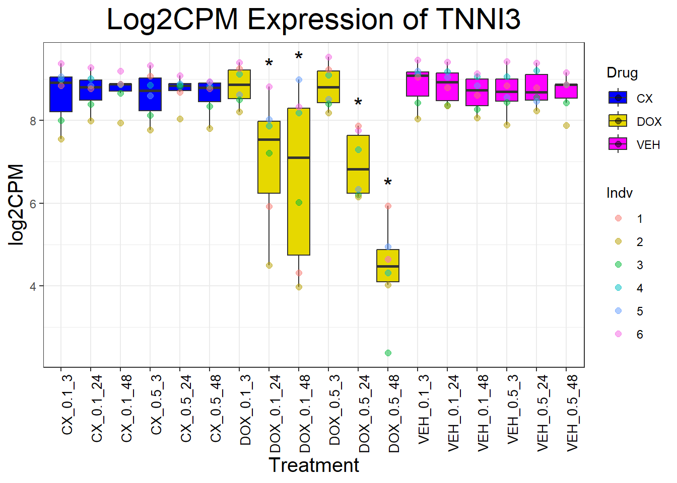
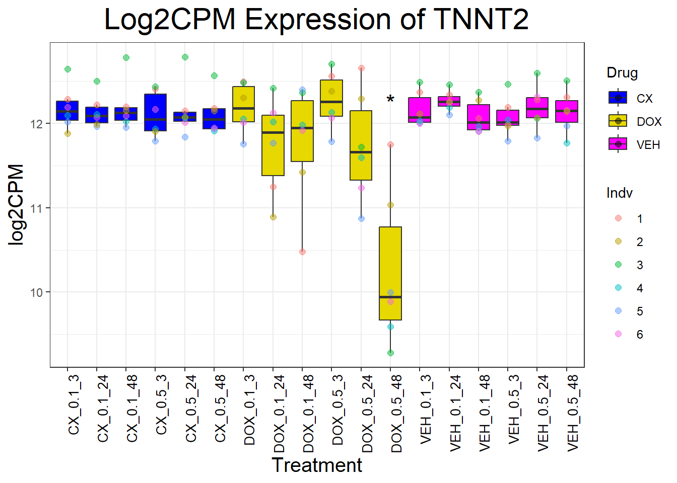
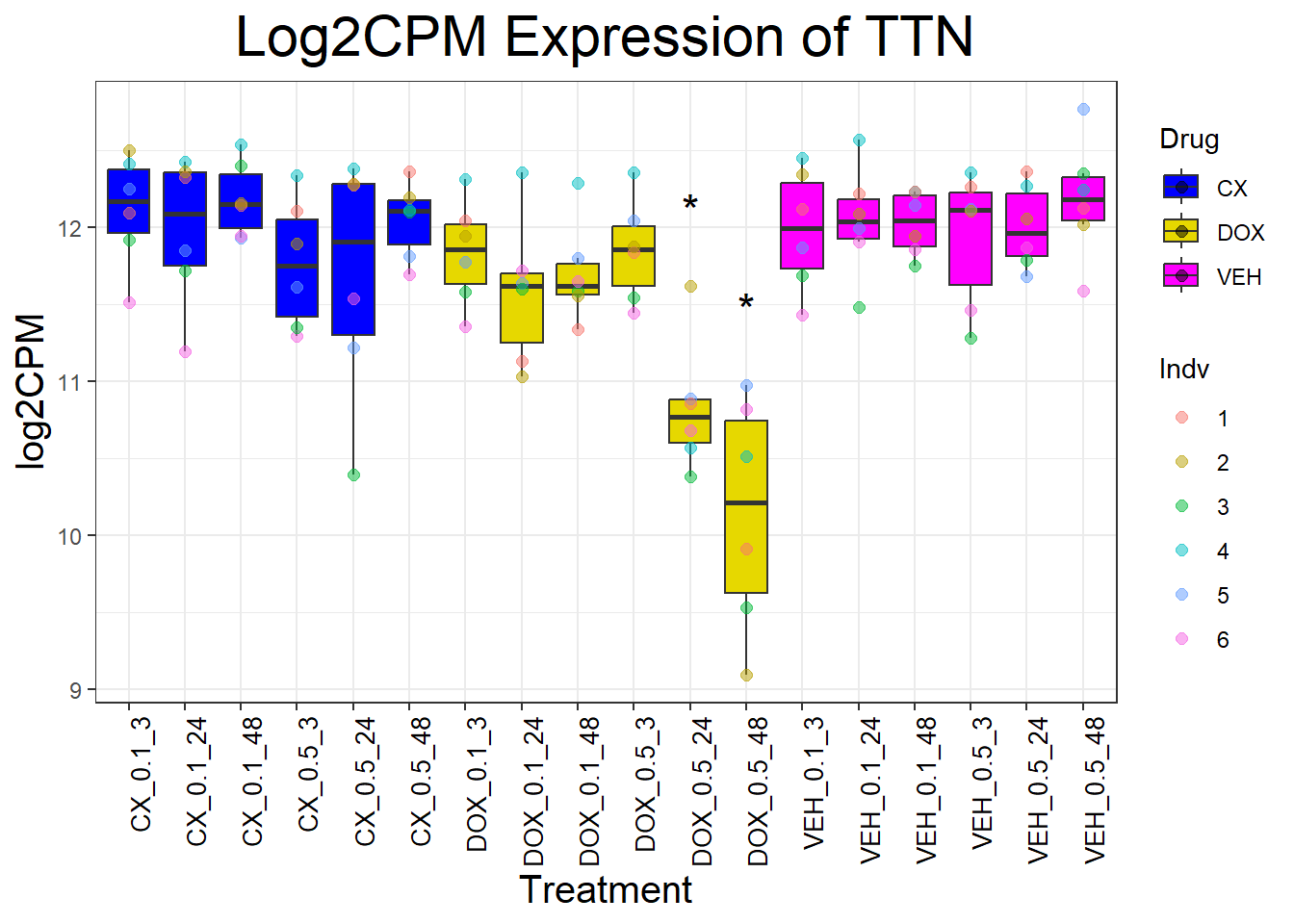
This analysis generates boxplots for cardiac genes and TOP2 genes across different treatments and timepoints.
📌 Load Required Libraries
library(ggplot2)Warning: package 'ggplot2' was built under R version 4.3.3library(dplyr)Warning: package 'dplyr' was built under R version 4.3.2library(tidyr)Warning: package 'tidyr' was built under R version 4.3.3library(org.Hs.eg.db)Warning: package 'AnnotationDbi' was built under R version 4.3.2Warning: package 'BiocGenerics' was built under R version 4.3.1Warning: package 'Biobase' was built under R version 4.3.1Warning: package 'IRanges' was built under R version 4.3.1Warning: package 'S4Vectors' was built under R version 4.3.1library(clusterProfiler)Warning: package 'clusterProfiler' was built under R version 4.3.3📌 Read Log2CPM Data
# Load feature count matrix
boxplot1 <- read.csv("data/Feature_count_Matrix_Log2CPM_filtered.csv") %>% as.data.frame()

# Ensure column names are cleaned
colnames(boxplot1) <- trimws(gsub("^X", "", colnames(boxplot1)))
📌 Define Genes of Interest
# Define the genes of interest
top2_genes <- c("TOP2A", "TOP2B")
cardiac_genes <- c("ACTN2", "CALR", "MYBPC3", "MYH6", "MYH7",
                   "MYL2", "RYR2", "SCN5A", "TNNI3", "TNNT2", "TTN")
dna_damage_genes <- c("TP53")  # Using correct gene symbol TP53
📌 Read and Process DEGs Data
# Load Toptables
deg_files <- list.files("data/DEGs", pattern = "Toptable_.*\\.csv", full.names = TRUE)
deg_list <- lapply(deg_files, read.csv)
names(deg_list) <- gsub("data/DEGs/Toptable_|\\.csv", "", deg_files)

# Function to check significance based on **Entrez_ID in the correct sample**
is_significant <- function(gene, drug, conc, timepoint) {
  condition <- paste(drug, conc, timepoint, sep = "_")
  if (!condition %in% names(deg_list)) return(FALSE)

  toptable <- deg_list[[condition]]
  gene_entrez <- boxplot1$ENTREZID[boxplot1$SYMBOL == gene]

  if (length(gene_entrez) == 0) return(FALSE)

  return(any(gene_entrez %in% toptable$Entrez_ID[toptable$adj.P.Val < 0.05]))
}
📌 Process Data for Plotting
process_gene_data <- function(gene) {
  # Filter log2CPM data for the gene
  gene_data <- boxplot1 %>% filter(SYMBOL == gene)

  # Reshape data
  long_data <- gene_data %>%
    pivot_longer(cols = -c(ENTREZID, SYMBOL, GENENAME), names_to = "Sample", values_to = "log2CPM") %>%
    mutate(
      Indv = case_when(
        grepl("75.1", Sample) ~ "1",
        grepl("78.1", Sample) ~ "2",
        grepl("87.1", Sample) ~ "3",
        grepl("17.3", Sample) ~ "4",
        grepl("84.1", Sample) ~ "5",
        grepl("90.1", Sample) ~ "6",
        TRUE ~ NA_character_
      ),
      Drug = case_when(
        grepl("CX.5461", Sample) ~ "CX",
        grepl("DOX", Sample) ~ "DOX",
        grepl("VEH", Sample) ~ "VEH",
        TRUE ~ NA_character_
      ),
      Conc. = case_when(
        grepl("_0.1_", Sample) ~ "0.1",
        grepl("_0.5_", Sample) ~ "0.5",
        TRUE ~ NA_character_
      ),
      Timepoint = case_when(
        grepl("_3$", Sample) ~ "3",
        grepl("_24$", Sample) ~ "24",
        grepl("_48$", Sample) ~ "48",
        TRUE ~ NA_character_
      ),
      Condition = paste(Drug, Conc., Timepoint, sep = "_")
    )

  # **Ensure Condition is Ordered Correctly**
  long_data$Condition <- factor(
    long_data$Condition,
    levels = c(
      "CX_0.1_3", "CX_0.1_24", "CX_0.1_48", "CX_0.5_3", "CX_0.5_24", "CX_0.5_48",
      "DOX_0.1_3", "DOX_0.1_24", "DOX_0.1_48", "DOX_0.5_3", "DOX_0.5_24", "DOX_0.5_48",
      "VEH_0.1_3", "VEH_0.1_24", "VEH_0.1_48", "VEH_0.5_3", "VEH_0.5_24", "VEH_0.5_48"
    )
  )

  # Identify significant conditions **per Drug, Conc, and Timepoint**
  significance_labels <- long_data %>%
    distinct(Drug, Conc., Timepoint, Condition) %>%
    rowwise() %>%
    mutate(
      max_log2CPM = max(long_data$log2CPM[long_data$Condition == Condition], na.rm = TRUE),
      Significance = ifelse(is_significant(gene, Drug, Conc., Timepoint), "*", "")
    ) %>%
    filter(Significance != "") %>% ungroup()

  list(long_data = long_data, significance_labels = significance_labels)
}
📌Generate Boxplots for Cardiac Genes
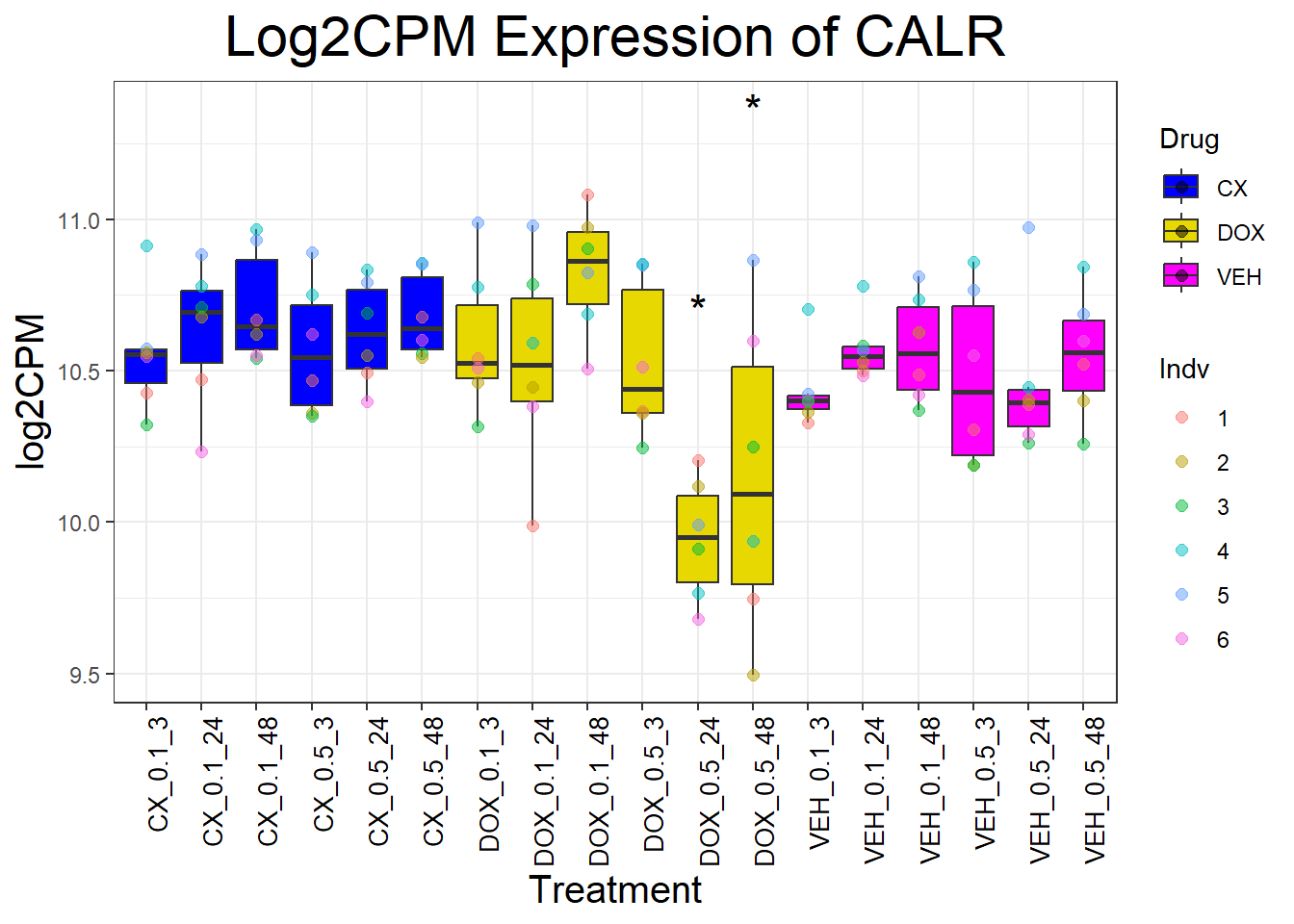
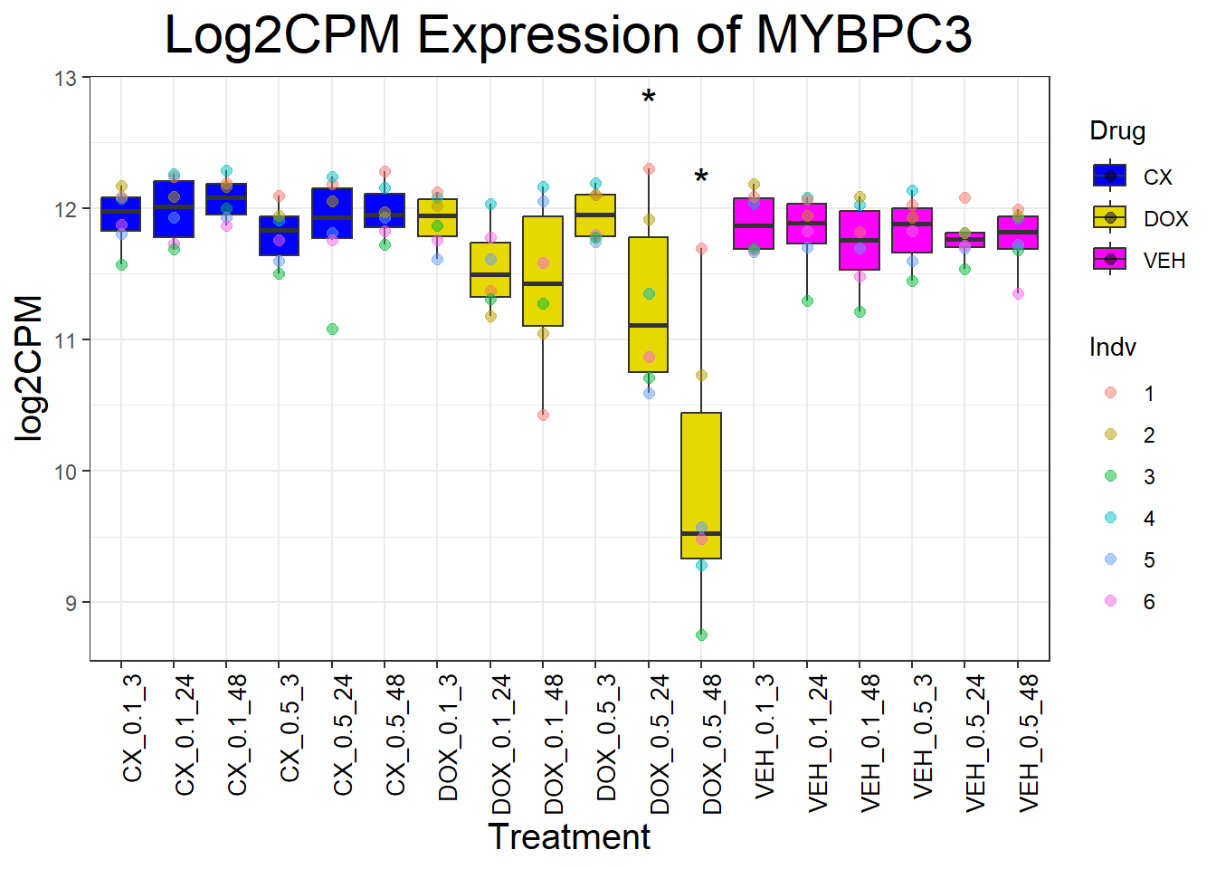
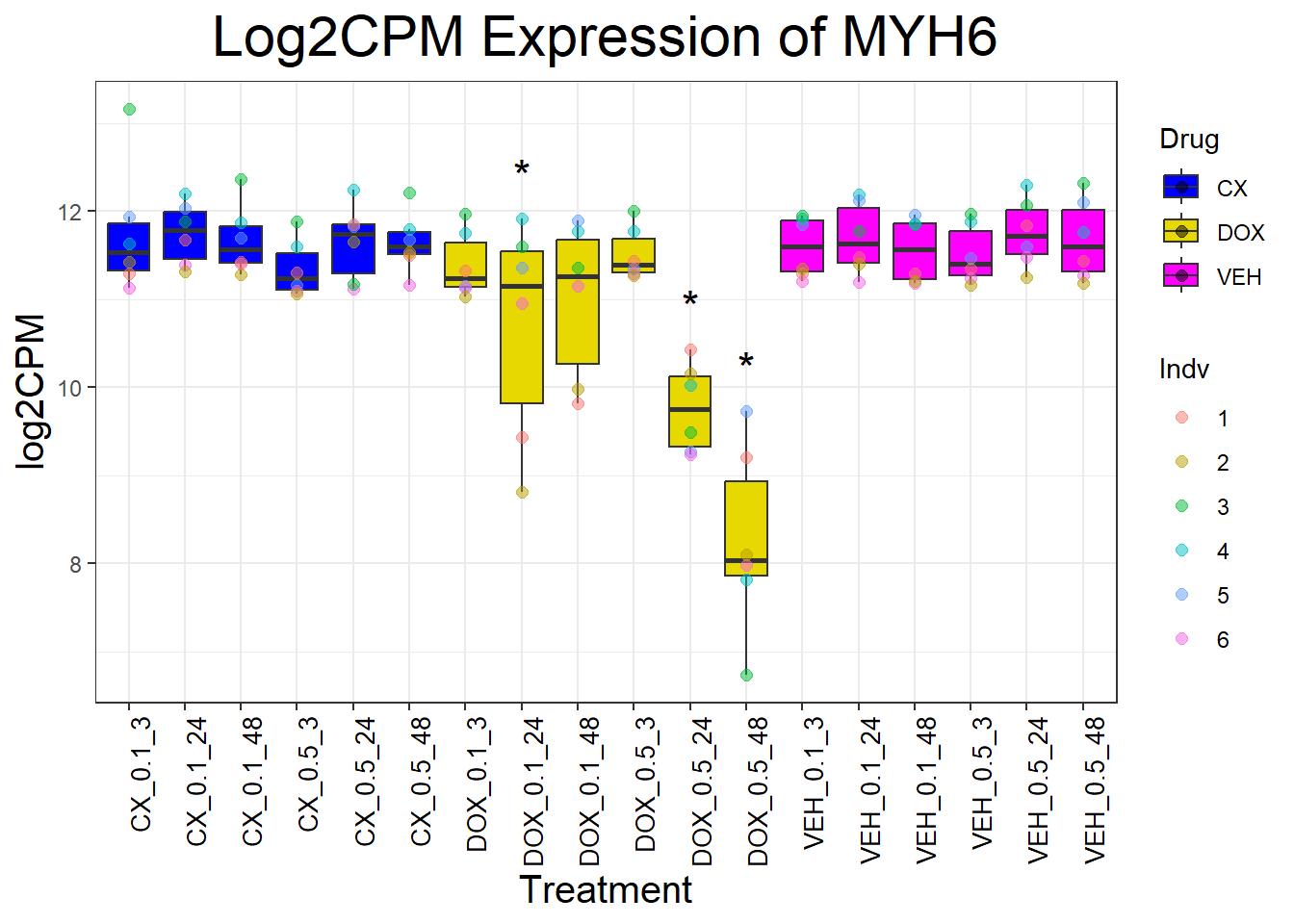
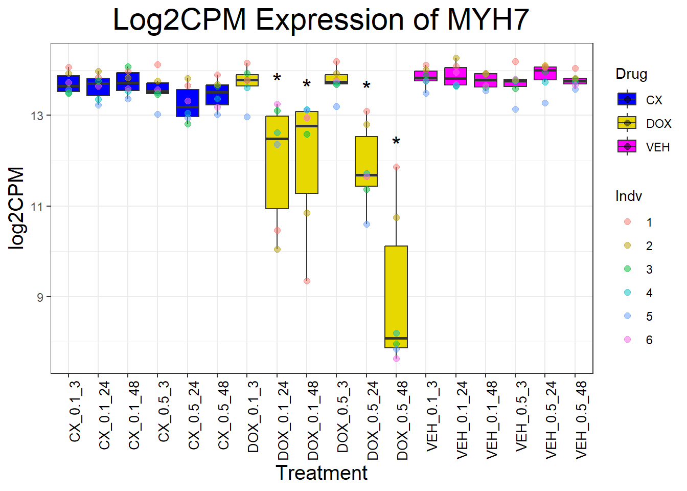
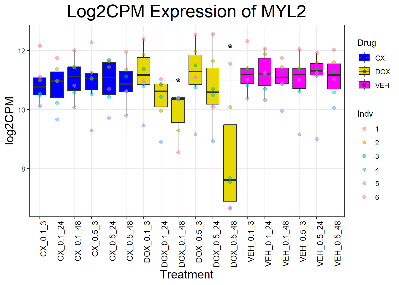
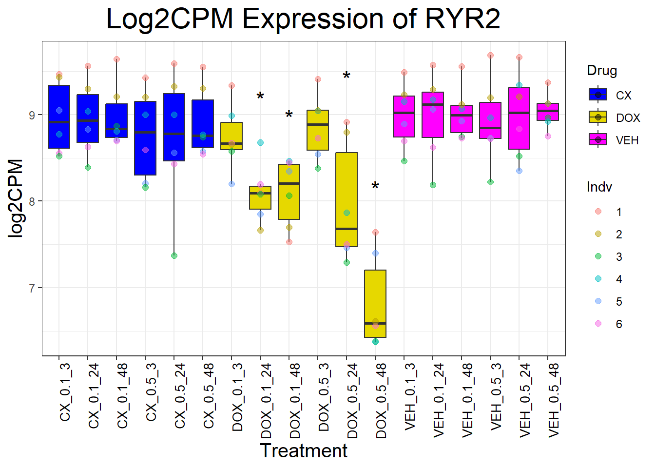
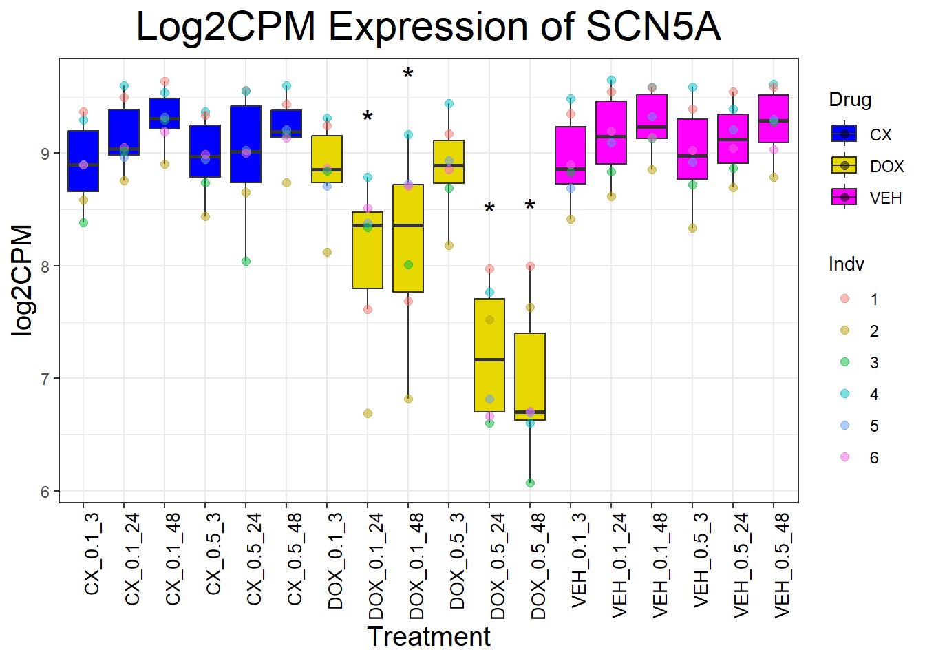
for (gene in cardiac_genes) {
  data_info <- process_gene_data(gene)
  p <- ggplot(data_info$long_data, aes(x = Condition, y = log2CPM, fill = Drug)) +
    geom_boxplot(outlier.shape = NA) +
    scale_fill_manual(values = c("CX" = "#0000FF", "DOX" = "#e6d800", "VEH" = "#FF00FF")) +
    geom_point(aes(color = Indv), size = 2, alpha = 0.5, position = position_jitter(width = -1, height = 0)) +
    geom_text(data = data_info$significance_labels, aes(x = Condition, y = max_log2CPM + 0.5, label = Significance),
              inherit.aes = FALSE, size = 6, color = "black") +
    ggtitle(paste("Log2CPM Expression of", gene)) +
    labs(x = "Treatment", y = "log2CPM") +
    theme_bw() +
    theme(plot.title = element_text(size = rel(2), hjust = 0.5),
          axis.title = element_text(size = 15, color = "black"),
          axis.text.x = element_text(size = 10, color = "black", angle = 90, hjust = 1))

  print(p)
}
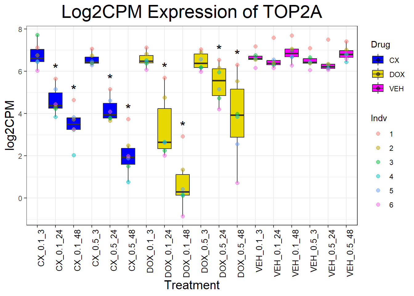
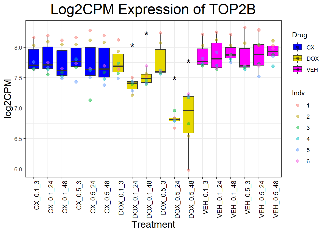
📌Generate Boxplots for TOP2 Genes
for (gene in top2_genes) {
  data_info <- process_gene_data(gene)
  p <- ggplot(data_info$long_data, aes(x = Condition, y = log2CPM, fill = Drug)) +
    geom_boxplot(outlier.shape = NA) +
    scale_fill_manual(values = c("CX" = "#0000FF", "DOX" = "#e6d800", "VEH" = "#FF00FF")) +
    geom_point(aes(color = Indv), size = 2, alpha = 0.5, position = position_jitter(width = -1, height = 0)) +
    geom_text(data = data_info$significance_labels, aes(x = Condition, y = max_log2CPM + 0.5, label = Significance),
              inherit.aes = FALSE, size = 6, color = "black") +
    ggtitle(paste("Log2CPM Expression of", gene)) +
    labs(x = "Treatment", y = "log2CPM") +
    theme_bw() +
    theme(plot.title = element_text(size = rel(2), hjust = 0.5),
          axis.title = element_text(size = 15, color = "black"),
          axis.text.x = element_text(size = 10, color = "black", angle = 90, hjust = 1))

  print(p)
}
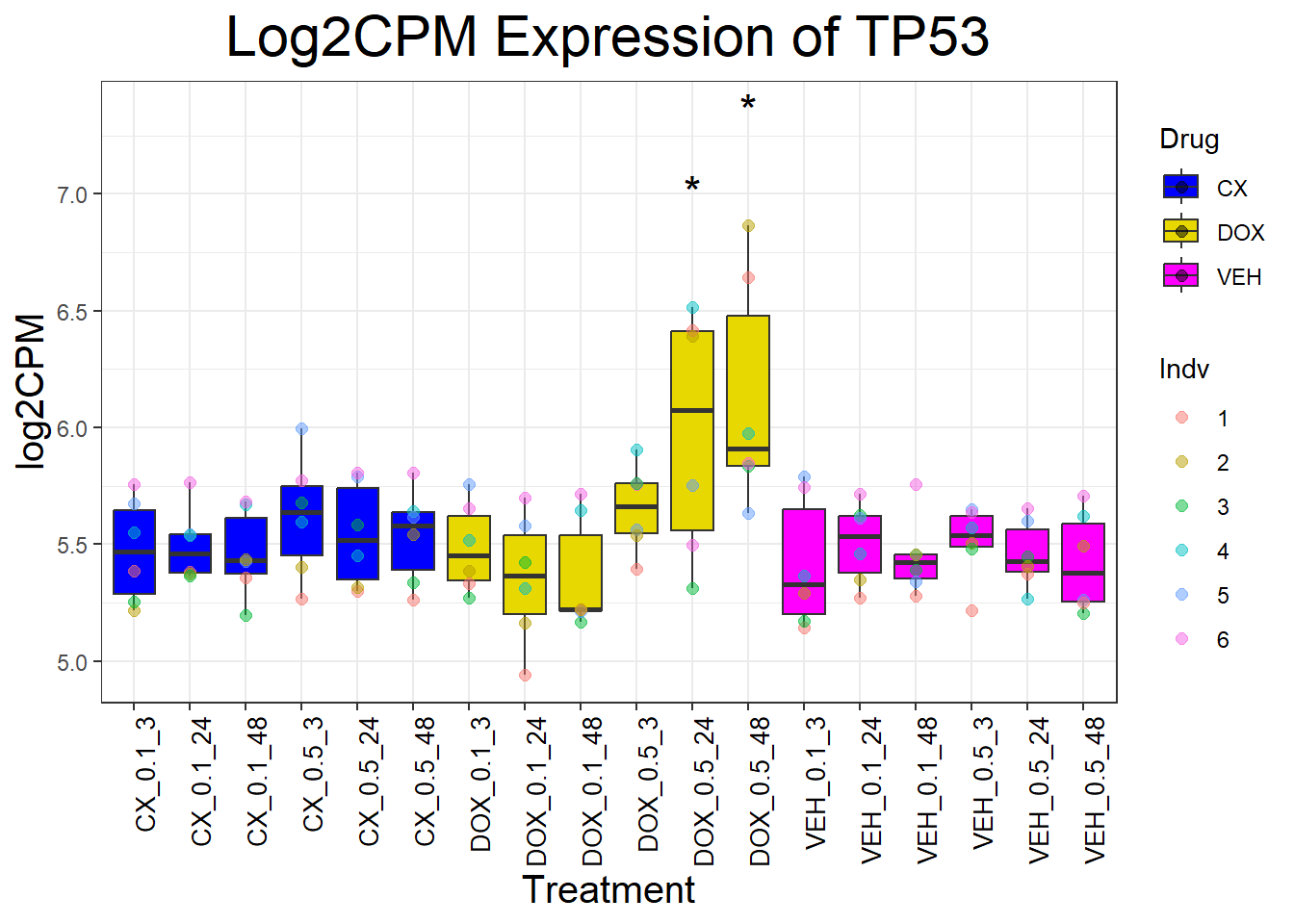
📌 Generate Boxplots for DNA Damage Genes
for (gene in dna_damage_genes) {
  data_info <- process_gene_data(gene)
  p <- ggplot(data_info$long_data, aes(x = Condition, y = log2CPM, fill = Drug)) +
    geom_boxplot(outlier.shape = NA) +
    scale_fill_manual(values = c("CX" = "#0000FF", "DOX" = "#e6d800", "VEH" = "#FF00FF")) +
    geom_point(aes(color = Indv), size = 2, alpha = 0.5, position = position_jitter(width = -1, height = 0)) +
    geom_text(data = data_info$significance_labels, aes(x = Condition, y = max_log2CPM + 0.5, label = Significance),
              inherit.aes = FALSE, size = 6, color = "black") +
    ggtitle(paste("Log2CPM Expression of", gene)) +
    labs(x = "Treatment", y = "log2CPM") +
    theme_bw() +
    theme(plot.title = element_text(size = rel(2), hjust = 0.5),
          axis.title = element_text(size = 15, color = "black"),
          axis.text.x = element_text(size = 10, color = "black", angle = 90, hjust = 1))

  print(p)
}
| Version | Author | Date |
|---|---|---|
| 456790a | sayanpaul01 | 2025-02-18 |
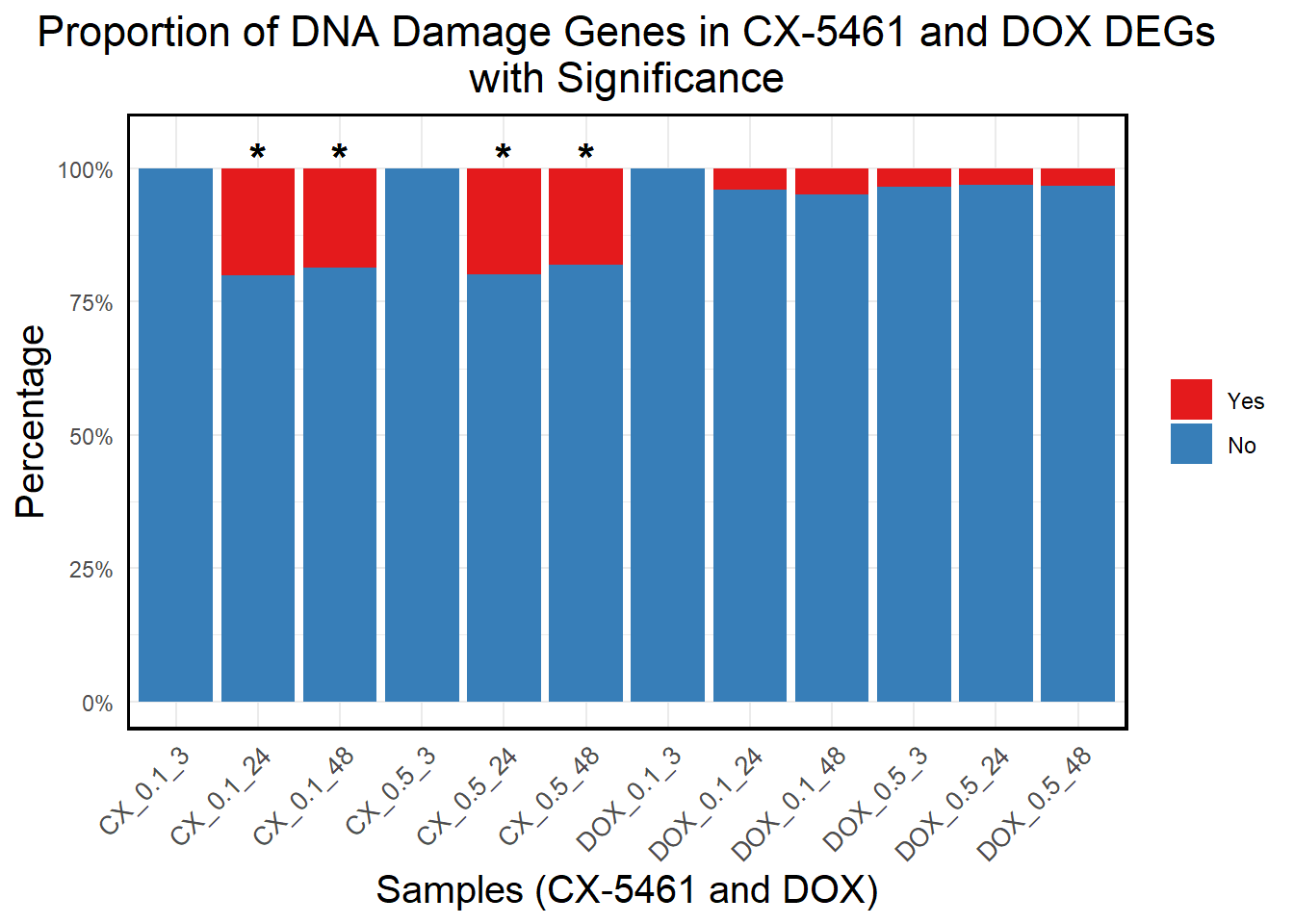
##📌 DNA Damage Proportion
📌 Read and Process DEG Data
# Load DEGs Data
CX_0.1_3 <- read.csv("data/DEGs/Toptable_CX_0.1_3.csv")
CX_0.1_24 <- read.csv("data/DEGs/Toptable_CX_0.1_24.csv")
CX_0.1_48 <- read.csv("data/DEGs/Toptable_CX_0.1_48.csv")
CX_0.5_3 <- read.csv("data/DEGs/Toptable_CX_0.5_3.csv")
CX_0.5_24 <- read.csv("data/DEGs/Toptable_CX_0.5_24.csv")
CX_0.5_48 <- read.csv("data/DEGs/Toptable_CX_0.5_48.csv")

DOX_0.1_3 <- read.csv("data/DEGs/Toptable_DOX_0.1_3.csv")
DOX_0.1_24 <- read.csv("data/DEGs/Toptable_DOX_0.1_24.csv")
DOX_0.1_48 <- read.csv("data/DEGs/Toptable_DOX_0.1_48.csv")
DOX_0.5_3 <- read.csv("data/DEGs/Toptable_DOX_0.5_3.csv")
DOX_0.5_24 <- read.csv("data/DEGs/Toptable_DOX_0.5_24.csv")
DOX_0.5_48 <- read.csv("data/DEGs/Toptable_DOX_0.5_48.csv")

# Extract Significant DEGs
DEGs <- list(
  "CX_0.1_3" = CX_0.1_3$Entrez_ID[CX_0.1_3$adj.P.Val < 0.05],
  "CX_0.1_24" = CX_0.1_24$Entrez_ID[CX_0.1_24$adj.P.Val < 0.05],
  "CX_0.1_48" = CX_0.1_48$Entrez_ID[CX_0.1_48$adj.P.Val < 0.05],
  "CX_0.5_3" = CX_0.5_3$Entrez_ID[CX_0.5_3$adj.P.Val < 0.05],
  "CX_0.5_24" = CX_0.5_24$Entrez_ID[CX_0.5_24$adj.P.Val < 0.05],
  "CX_0.5_48" = CX_0.5_48$Entrez_ID[CX_0.5_48$adj.P.Val < 0.05],
  "DOX_0.1_3" = DOX_0.1_3$Entrez_ID[DOX_0.1_3$adj.P.Val < 0.05],
  "DOX_0.1_24" = DOX_0.1_24$Entrez_ID[DOX_0.1_24$adj.P.Val < 0.05],
  "DOX_0.1_48" = DOX_0.1_48$Entrez_ID[DOX_0.1_48$adj.P.Val < 0.05],
  "DOX_0.5_3" = DOX_0.5_3$Entrez_ID[DOX_0.5_3$adj.P.Val < 0.05],
  "DOX_0.5_24" = DOX_0.5_24$Entrez_ID[DOX_0.5_24$adj.P.Val < 0.05],
  "DOX_0.5_48" = DOX_0.5_48$Entrez_ID[DOX_0.5_48$adj.P.Val < 0.05]
)

# Extract Significant DEGs
DEG1 <- CX_0.1_3$Entrez_ID[CX_0.1_3$adj.P.Val < 0.05]
DEG2 <- CX_0.1_24$Entrez_ID[CX_0.1_24$adj.P.Val < 0.05]
DEG3 <- CX_0.1_48$Entrez_ID[CX_0.1_48$adj.P.Val < 0.05]
DEG4 <- CX_0.5_3$Entrez_ID[CX_0.5_3$adj.P.Val < 0.05]
DEG5 <- CX_0.5_24$Entrez_ID[CX_0.5_24$adj.P.Val < 0.05]
DEG6 <- CX_0.5_48$Entrez_ID[CX_0.5_48$adj.P.Val < 0.05]

DEG7 <- DOX_0.1_3$Entrez_ID[DOX_0.1_3$adj.P.Val < 0.05]
DEG8 <- DOX_0.1_24$Entrez_ID[DOX_0.1_24$adj.P.Val < 0.05]
DEG9 <- DOX_0.1_48$Entrez_ID[DOX_0.1_48$adj.P.Val < 0.05]
DEG10 <- DOX_0.5_3$Entrez_ID[DOX_0.5_3$adj.P.Val < 0.05]
DEG11 <- DOX_0.5_24$Entrez_ID[DOX_0.5_24$adj.P.Val < 0.05]
DEG12 <- DOX_0.5_48$Entrez_ID[DOX_0.5_48$adj.P.Val < 0.05]
📌 DNA Damage Proportion with Chi-Square Test
# Load DNA Damage Genes List
DNA_damage <- read.csv("data/DNA_Damage.csv", stringsAsFactors = FALSE)
DNA_damage$Entrez_ID <- mapIds(org.Hs.eg.db,
                               keys = DNA_damage$Symbol,
                               column = "ENTREZID",
                               keytype = "SYMBOL",
                               multiVals = "first")

# Define CX-5461 DEG lists
CX_DEGs <- list(
  "CX_0.1_3" = DEG1, "CX_0.1_24" = DEG2, "CX_0.1_48" = DEG3,
  "CX_0.5_3" = DEG4, "CX_0.5_24" = DEG5, "CX_0.5_48" = DEG6
)

# Define DOX DEG lists
DOX_DEGs <- list(
  "DOX_0.1_3" = DEG7, "DOX_0.1_24" = DEG8, "DOX_0.1_48" = DEG9,
  "DOX_0.5_3" = DEG10, "DOX_0.5_24" = DEG11, "DOX_0.5_48" = DEG12
)

# Extract Entrez_IDs from DNA Damage gene dataset
DNA_damage_genes <- na.omit(DNA_damage$Entrez_ID)

# Combine CX-5461 DEGs into a dataframe with a "Drug" column
CX_DEGs_df <- bind_rows(
  lapply(CX_DEGs, function(ids) data.frame(Entrez_ID = ids, Drug = "CX-5461")),
  .id = "Sample"
)

# Combine DOX DEGs into a dataframe with a "Drug" column
DOX_DEGs_df <- bind_rows(
  lapply(DOX_DEGs, function(ids) data.frame(Entrez_ID = ids, Drug = "DOX")),
  .id = "Sample"
)

# Merge CX-5461 and DOX datasets
DEGs_df <- bind_rows(CX_DEGs_df, DOX_DEGs_df)

# Check if genes are in DNA Damage list
DEGs_df <- DEGs_df %>%
  mutate(Category = ifelse(Entrez_ID %in% DNA_damage_genes, "Yes", "No"))

# Count DNA damage genes in each sample
proportion_data <- DEGs_df %>%
  group_by(Sample, Drug, Category) %>%
  summarise(Count = n(), .groups = "drop") %>%
  group_by(Sample, Drug) %>%
  mutate(Percentage = (Count / sum(Count)) * 100)

# Normalize Percentages to Sum Exactly 100%
proportion_data <- proportion_data %>%
  group_by(Sample) %>%
  mutate(Percentage = round(Percentage, 2)) %>%
  mutate(Adjustment = 100 - sum(Percentage, na.rm = TRUE)) %>%
  mutate(Percentage = ifelse(Category == "No", Percentage + Adjustment, Percentage)) %>%
  mutate(Percentage = ifelse(Percentage < 0, 0, Percentage)) %>%
  mutate(Percentage = ifelse(Percentage > 100, 100, Percentage)) %>%
  ungroup() %>%
  replace_na(list(Percentage = 0))

# Ensure "Yes" is at the Bottom and "No" is at the Top
proportion_data$Category <- factor(proportion_data$Category, levels = c("Yes", "No"))

# **🔹 Maintain Correct X-Axis Order (3 → 24 → 48)**
sample_order <- c(
  "CX_0.1_3", "CX_0.1_24", "CX_0.1_48",
  "CX_0.5_3", "CX_0.5_24", "CX_0.5_48",
  "DOX_0.1_3", "DOX_0.1_24", "DOX_0.1_48",
  "DOX_0.5_3", "DOX_0.5_24", "DOX_0.5_48"
)
proportion_data$Sample <- factor(proportion_data$Sample, levels = sample_order, ordered = TRUE)

# **Perform Chi-Square Test for CX vs DOX Pairs**
chi_square_results <- data.frame(Sample = character(), P_Value = numeric())

for (i in seq(1, 6)) {  # Pairwise comparison (CX vs DOX)
  cx_sample <- sample_order[i]
  dox_sample <- sample_order[i + 6]  # Correctly pairs CX_0.1_3 with DOX_0.1_3, etc.

  cx_data <- filter(proportion_data, Sample == cx_sample)
  dox_data <- filter(proportion_data, Sample == dox_sample)

  # Construct contingency table for Chi-Square test
  contingency_table <- matrix(
    c(sum(cx_data$Count[cx_data$Category == "Yes"]), sum(cx_data$Count[cx_data$Category == "No"]),
      sum(dox_data$Count[dox_data$Category == "Yes"]), sum(dox_data$Count[dox_data$Category == "No"])),
    nrow = 2, byrow = TRUE
  )

  # Run Chi-Square Test
  test_result <- chisq.test(contingency_table)
  p_value <- test_result$p.value

  # Store results
  chi_square_results <- rbind(chi_square_results, data.frame(Sample = cx_sample, P_Value = p_value))
}

# Identify significant CX samples (p < 0.05)
chi_square_results$Significant <- ifelse(chi_square_results$P_Value < 0.05, "*", "")

# **🔹 Merge Chi-Square Results WITHOUT Modifying Order**
proportion_data <- left_join(proportion_data, chi_square_results, by = "Sample")

# **Reapply Factor Order to Prevent Changes**
proportion_data$Sample <- factor(proportion_data$Sample, levels = sample_order, ordered = TRUE)
📌 DNA Damage Proportion Plot
# **Generate Proportion Plot for CX-5461 and DOX**
ggplot(proportion_data, aes(x = Sample, y = Percentage, fill = Category)) +
  geom_bar(stat = "identity", position = "stack") +
  geom_text(data = subset(proportion_data, Significant == "*"),
            aes(x = Sample, y = 102, label = "*"),
            size = 6, color = "black", fontface = "bold") +
  scale_y_continuous(labels = scales::percent_format(scale = 1), limits = c(0, 105)) +
  scale_fill_manual(values = c("Yes" = "#e41a1c", "No" = "#377eb8")) +
  labs(
    title = "Proportion of DNA Damage Genes in CX-5461 and DOX DEGs\nwith Significance",
    x = "Samples (CX-5461 and DOX)",
    y = "Percentage",
    fill = "Category"
  ) +
  theme_minimal() +
  theme(
    plot.title = element_text(size = rel(1.5), hjust = 0.5),
    axis.title = element_text(size = 15, color = "black"),
    axis.text.x = element_text(size = 10, angle = 45, hjust = 1),
    legend.title = element_blank(),
    panel.border = element_rect(color = "black", fill = NA, linewidth = 1.2),
    strip.background = element_blank(),
    strip.text = element_text(size = 12, face = "bold")
  )
sessionInfo()R version 4.3.0 (2023-04-21 ucrt)
Platform: x86_64-w64-mingw32/x64 (64-bit)
Running under: Windows 11 x64 (build 22631)
Matrix products: default
locale:
[1] LC_COLLATE=English_United States.utf8
[2] LC_CTYPE=English_United States.utf8
[3] LC_MONETARY=English_United States.utf8
[4] LC_NUMERIC=C
[5] LC_TIME=English_United States.utf8
time zone: America/Chicago
tzcode source: internal
attached base packages:
[1] stats4 stats graphics grDevices utils datasets methods
[8] base
other attached packages:
[1] clusterProfiler_4.10.1 org.Hs.eg.db_3.18.0 AnnotationDbi_1.64.1
[4] IRanges_2.36.0 S4Vectors_0.40.1 Biobase_2.62.0
[7] BiocGenerics_0.48.1 tidyr_1.3.1 dplyr_1.1.4
[10] ggplot2_3.5.1 workflowr_1.7.1
loaded via a namespace (and not attached):
[1] DBI_1.2.3 bitops_1.0-7 gson_0.1.0
[4] shadowtext_0.1.4 gridExtra_2.3 rlang_1.1.3
[7] magrittr_2.0.3 DOSE_3.28.2 git2r_0.35.0
[10] compiler_4.3.0 RSQLite_2.3.3 getPass_0.2-4
[13] png_0.1-8 callr_3.7.6 vctrs_0.6.5
[16] reshape2_1.4.4 stringr_1.5.1 pkgconfig_2.0.3
[19] crayon_1.5.3 fastmap_1.1.1 XVector_0.42.0
[22] labeling_0.4.3 ggraph_2.2.1 HDO.db_0.99.1
[25] promises_1.3.0 rmarkdown_2.29 enrichplot_1.22.0
[28] ps_1.8.1 purrr_1.0.2 bit_4.0.5
[31] xfun_0.50 zlibbioc_1.48.0 cachem_1.0.8
[34] aplot_0.2.3 GenomeInfoDb_1.38.8 jsonlite_1.8.9
[37] blob_1.2.4 later_1.3.2 BiocParallel_1.36.0
[40] tweenr_2.0.3 parallel_4.3.0 R6_2.5.1
[43] RColorBrewer_1.1-3 bslib_0.8.0 stringi_1.8.3
[46] jquerylib_0.1.4 GOSemSim_2.28.1 Rcpp_1.0.12
[49] knitr_1.49 httpuv_1.6.15 Matrix_1.6-1.1
[52] splines_4.3.0 igraph_2.1.1 tidyselect_1.2.1
[55] viridis_0.6.5 qvalue_2.34.0 rstudioapi_0.17.1
[58] yaml_2.3.10 codetools_0.2-20 processx_3.8.5
[61] lattice_0.22-5 tibble_3.2.1 plyr_1.8.9
[64] treeio_1.26.0 withr_3.0.2 KEGGREST_1.42.0
[67] evaluate_1.0.3 gridGraphics_0.5-1 scatterpie_0.2.4
[70] polyclip_1.10-7 Biostrings_2.70.1 ggtree_3.10.1
[73] pillar_1.10.1 whisker_0.4.1 ggfun_0.1.8
[76] generics_0.1.3 rprojroot_2.0.4 RCurl_1.98-1.13
[79] tidytree_0.4.6 munsell_0.5.1 scales_1.3.0
[82] glue_1.7.0 lazyeval_0.2.2 tools_4.3.0
[85] data.table_1.14.10 fgsea_1.28.0 fs_1.6.3
[88] graphlayouts_1.2.0 fastmatch_1.1-4 tidygraph_1.3.1
[91] cowplot_1.1.3 grid_4.3.0 ape_5.8
[94] colorspace_2.1-0 nlme_3.1-166 patchwork_1.3.0
[97] GenomeInfoDbData_1.2.11 ggforce_0.4.2 cli_3.6.1
[100] viridisLite_0.4.2 gtable_0.3.6 yulab.utils_0.1.8
[103] sass_0.4.9 digest_0.6.34 ggplotify_0.1.2
[106] ggrepel_0.9.6 farver_2.1.2 memoise_2.0.1
[109] htmltools_0.5.8.1 lifecycle_1.0.4 httr_1.4.7
[112] GO.db_3.18.0 bit64_4.0.5 MASS_7.3-60