Corrmotif Conc Analysis

workflowr

• Summary
• Checks
• Past versions

Last updated: 2025-03-10

Checks: 6 1

Knit directory: CX5461_Project/

This reproducible R Markdown analysis was created with workflowr (version 1.7.1). The Checks tab describes the reproducibility checks that were applied when the results were created. The Past versions tab lists the development history.

---

R Markdown file: uncommitted changes

The R Markdown file has unstaged changes. To know which version of the R Markdown file created these results, you’ll want to first commit it to the Git repo. If you’re still working on the analysis, you can ignore this warning. When you’re finished, you can run wflow_publish to commit the R Markdown file and build the HTML.

Environment: empty

Great job! The global environment was empty. Objects defined in the global environment can affect the analysis in your R Markdown file in unknown ways. For reproduciblity it’s best to always run the code in an empty environment.

Seed: set.seed(20250129)

The command set.seed(20250129) was run prior to running the code in the R Markdown file. Setting a seed ensures that any results that rely on randomness, e.g. subsampling or permutations, are reproducible.

Session information: recorded

Great job! Recording the operating system, R version, and package versions is critical for reproducibility.

Cache: none

Nice! There were no cached chunks for this analysis, so you can be confident that you successfully produced the results during this run.

File paths: relative

Great job! Using relative paths to the files within your workflowr project makes it easier to run your code on other machines.

Repository version: 282d854

Great! You are using Git for version control. Tracking code development and connecting the code version to the results is critical for reproducibility.

The results in this page were generated with repository version 282d854. See the Past versions tab to see a history of the changes made to the R Markdown and HTML files.

Note that you need to be careful to ensure that all relevant files for the analysis have been committed to Git prior to generating the results (you can use wflow_publish or wflow_git_commit). workflowr only checks the R Markdown file, but you know if there are other scripts or data files that it depends on. Below is the status of the Git repository when the results were generated:

Ignored files:
    Ignored:    .RData
    Ignored:    .Rhistory
    Ignored:    .Rproj.user/

Unstaged changes:
    Modified:   analysis/Corrmotif_Conc.Rmd

Note that any generated files, e.g. HTML, png, CSS, etc., are not included in this status report because it is ok for generated content to have uncommitted changes.

---

These are the previous versions of the repository in which changes were made to the R Markdown (analysis/Corrmotif_Conc.Rmd) and HTML (docs/Corrmotif_Conc.html) files. If you’ve configured a remote Git repository (see ?wflow_git_remote), click on the hyperlinks in the table below to view the files as they were in that past version.

File	Version	Author	Date	Message
Rmd	ef3a951	sayanpaul01	2025-03-09	Commit
html	ef3a951	sayanpaul01	2025-03-09	Commit
Rmd	81247f6	sayanpaul01	2025-03-06	Commit
html	81247f6	sayanpaul01	2025-03-06	Commit
Rmd	96d0db1	sayanpaul01	2025-03-05	Commit
html	96d0db1	sayanpaul01	2025-03-05	Commit
Rmd	91a7ce4	sayanpaul01	2025-03-03	Commit
html	91a7ce4	sayanpaul01	2025-03-03	Commit
Rmd	d9ff853	sayanpaul01	2025-03-03	Commit
html	d9ff853	sayanpaul01	2025-03-03	Commit
Rmd	2de67e6	sayanpaul01	2025-02-27	Commit
html	2de67e6	sayanpaul01	2025-02-27	Commit
Rmd	41cd1be	sayanpaul01	2025-02-27	Commit
html	41cd1be	sayanpaul01	2025-02-27	Commit
Rmd	f84821f	sayanpaul01	2025-02-26	Commit
Rmd	b6e38a1	sayanpaul01	2025-02-25	Commit
html	b6e38a1	sayanpaul01	2025-02-25	Commit
Rmd	ce4b325	sayanpaul01	2025-02-25	Commit
html	ce4b325	sayanpaul01	2025-02-25	Commit

---

📌 0.1 Micromolar

📌 Fit Limma Model Functions

## Fit limma model using code as it is found in the original cormotif code. It has
## only been modified to add names to the matrix of t values, as well as the
## limma fits

limmafit.default <- function(exprs,groupid,compid) {
  limmafits  <- list()
  compnum    <- nrow(compid)
  genenum    <- nrow(exprs)
  limmat     <- matrix(0,genenum,compnum)
  limmas2    <- rep(0,compnum)
  limmadf    <- rep(0,compnum)
  limmav0    <- rep(0,compnum)
  limmag1num <- rep(0,compnum)
  limmag2num <- rep(0,compnum)

  rownames(limmat)  <- rownames(exprs)
  colnames(limmat)  <- rownames(compid)
  names(limmas2)    <- rownames(compid)
  names(limmadf)    <- rownames(compid)
  names(limmav0)    <- rownames(compid)
  names(limmag1num) <- rownames(compid)
  names(limmag2num) <- rownames(compid)

  for(i in 1:compnum) {
    selid1 <- which(groupid == compid[i,1])
    selid2 <- which(groupid == compid[i,2])
    eset   <- new("ExpressionSet", exprs=cbind(exprs[,selid1],exprs[,selid2]))
    g1num  <- length(selid1)
    g2num  <- length(selid2)
    designmat <- cbind(base=rep(1,(g1num+g2num)), delta=c(rep(0,g1num),rep(1,g2num)))
    fit <- lmFit(eset,designmat)
    fit <- eBayes(fit)
    limmat[,i] <- fit$t[,2]
    limmas2[i] <- fit$s2.prior
    limmadf[i] <- fit$df.prior
    limmav0[i] <- fit$var.prior[2]
    limmag1num[i] <- g1num
    limmag2num[i] <- g2num
    limmafits[[i]] <- fit

    # log odds
    # w<-sqrt(1+fit$var.prior[2]/(1/g1num+1/g2num))
    # log(0.99)+dt(fit$t[1,2],g1num+g2num-2+fit$df.prior,log=TRUE)-log(0.01)-dt(fit$t[1,2]/w, g1num+g2num-2+fit$df.prior, log=TRUE)+log(w)
  }
  names(limmafits) <- rownames(compid)
  limmacompnum<-nrow(compid)
  result<-list(t       = limmat,
               v0      = limmav0,
               df0     = limmadf,
               s20     = limmas2,
               g1num   = limmag1num,
               g2num   = limmag2num,
               compnum = limmacompnum,
               fits    = limmafits)
}

limmafit.counts <-
  function (exprs, groupid, compid, norm.factor.method = "TMM", voom.normalize.method = "none")
  {
    limmafits  <- list()
    compnum    <- nrow(compid)
    genenum    <- nrow(exprs)
    limmat     <- matrix(NA,genenum,compnum)
    limmas2    <- rep(0,compnum)
    limmadf    <- rep(0,compnum)
    limmav0    <- rep(0,compnum)
    limmag1num <- rep(0,compnum)
    limmag2num <- rep(0,compnum)

    rownames(limmat)  <- rownames(exprs)
    colnames(limmat)  <- rownames(compid)
    names(limmas2)    <- rownames(compid)
    names(limmadf)    <- rownames(compid)
    names(limmav0)    <- rownames(compid)
    names(limmag1num) <- rownames(compid)
    names(limmag2num) <- rownames(compid)

    for (i in 1:compnum) {
      message(paste("Running limma for comparision",i,"/",compnum))
      selid1 <- which(groupid == compid[i, 1])
      selid2 <- which(groupid == compid[i, 2])
      # make a new count data frame
      counts <- cbind(exprs[, selid1], exprs[, selid2])

      # remove NAs
      not.nas <- which(apply(counts, 1, function(x) !any(is.na(x))) == TRUE)

      # runn voom/limma
      d <- DGEList(counts[not.nas,])
      d <- calcNormFactors(d, method = norm.factor.method)
      g1num <- length(selid1)
      g2num <- length(selid2)
      designmat <- cbind(base = rep(1, (g1num + g2num)), delta = c(rep(0,
                                                                       g1num), rep(1, g2num)))

      y <- voom(d, designmat, normalize.method = voom.normalize.method)
      fit <- lmFit(y, designmat)
      fit <- eBayes(fit)

      limmafits[[i]] <- fit
      limmat[not.nas, i] <- fit$t[, 2]
      limmas2[i] <- fit$s2.prior
      limmadf[i] <- fit$df.prior
      limmav0[i] <- fit$var.prior[2]
      limmag1num[i] <- g1num
      limmag2num[i] <- g2num
    }
    limmacompnum <- nrow(compid)
    names(limmafits) <- rownames(compid)
    result <- list(t       = limmat,
                   v0      = limmav0,
                   df0     = limmadf,
                   s20     = limmas2,
                   g1num   = limmag1num,
                   g2num   = limmag2num,
                   compnum = limmacompnum,
                   fits    = limmafits)
  }

limmafit.list <-
  function (fitlist, cmp.idx=2)
  {
    compnum    <- length(fitlist)

    genes <- c()
    for (i in 1:compnum) genes <- unique(c(genes, rownames(fitlist[[i]])))

    genenum    <- length(genes)
    limmat     <- matrix(NA,genenum,compnum)
    limmas2    <- rep(0,compnum)
    limmadf    <- rep(0,compnum)
    limmav0    <- rep(0,compnum)
    limmag1num <- rep(0,compnum)
    limmag2num <- rep(0,compnum)

    rownames(limmat)  <- genes
    colnames(limmat)  <- names(fitlist)
    names(limmas2)    <- names(fitlist)
    names(limmadf)    <- names(fitlist)
    names(limmav0)    <- names(fitlist)
    names(limmag1num) <- names(fitlist)
    names(limmag2num) <- names(fitlist)

    for (i in 1:compnum) {
      this.t <- fitlist[[i]]$t[,cmp.idx]
      limmat[names(this.t),i] <- this.t

      limmas2[i]    <- fitlist[[i]]$s2.prior
      limmadf[i]    <- fitlist[[i]]$df.prior
      limmav0[i]    <- fitlist[[i]]$var.prior[cmp.idx]
      limmag1num[i] <- sum(fitlist[[i]]$design[,cmp.idx]==0)
      limmag2num[i] <- sum(fitlist[[i]]$design[,cmp.idx]==1)
    }

    limmacompnum <- compnum
    result <- list(t       = limmat,
                   v0      = limmav0,
                   df0     = limmadf,
                   s20     = limmas2,
                   g1num   = limmag1num,
                   g2num   = limmag2num,
                   compnum = limmacompnum,
                   fits    = limmafits)

  }

## Rank genes based on statistics
generank<-function(x) {
  xcol<-ncol(x)
  xrow<-nrow(x)
  result<-matrix(0,xrow,xcol)
  z<-(1:1:xrow)
  for(i in 1:xcol) {
    y<-sort(x[,i],decreasing=TRUE,na.last=TRUE)
    result[,i]<-match(x[,i],y)
    result[,i]<-order(result[,i])
  }
  result
}

## Log-likelihood for moderated t under H0
modt.f0.loglike<-function(x,df) {
  a<-dt(x, df, log=TRUE)
  result<-as.vector(a)
  flag<-which(is.na(result)==TRUE)
  result[flag]<-0
  result
}

## Log-likelihood for moderated t under H1
## param=c(df,g1num,g2num,v0)
modt.f1.loglike<-function(x,param) {
  df<-param[1]
  g1num<-param[2]
  g2num<-param[3]
  v0<-param[4]
  w<-sqrt(1+v0/(1/g1num+1/g2num))
  dt(x/w, df, log=TRUE)-log(w)
  a<-dt(x/w, df, log=TRUE)-log(w)
  result<-as.vector(a)
  flag<-which(is.na(result)==TRUE)
  result[flag]<-0
  result
}

## Correlation Motif Fit
cmfit.X<-function(x, type, K=1, tol=1e-3, max.iter=100) {
  ## initialize
  xrow <- nrow(x)
  xcol <- ncol(x)
  loglike0 <- list()
  loglike1 <- list()
  p <- rep(1, K)/K
  q <- matrix(runif(K * xcol), K, xcol)
  q[1, ] <- rep(0.01, xcol)
  for (i in 1:xcol) {
    f0 <- type[[i]][[1]]
    f0param <- type[[i]][[2]]
    f1 <- type[[i]][[3]]
    f1param <- type[[i]][[4]]
    loglike0[[i]] <- f0(x[, i], f0param)
    loglike1[[i]] <- f1(x[, i], f1param)
  }
  condlike <- list()
  for (i in 1:xcol) {
    condlike[[i]] <- matrix(0, xrow, K)
  }
  loglike.old <- -1e+10
  for (i.iter in 1:max.iter) {
    if ((i.iter%%50) == 0) {
      print(paste("We have run the first ", i.iter, " iterations for K=",
                  K, sep = ""))
    }
    err <- tol + 1
    clustlike <- matrix(0, xrow, K)
    #templike <- matrix(0, xrow, 2)
    templike1 <- rep(0, xrow)
    templike2 <- rep(0, xrow)
    for (j in 1:K) {
      for (i in 1:xcol) {
        templike1 <- log(q[j, i]) + loglike1[[i]]
        templike2 <- log(1 - q[j, i]) + loglike0[[i]]
        tempmax <- Rfast::Pmax(templike1, templike2)

        templike1 <- exp(templike1 - tempmax)
        templike2 <- exp(templike2 - tempmax)

        tempsum <- templike1 + templike2
        clustlike[, j] <- clustlike[, j] + tempmax +
          log(tempsum)
        condlike[[i]][, j] <- templike1/tempsum
      }
      clustlike[, j] <- clustlike[, j] + log(p[j])
    }
    #tempmax <- apply(clustlike, 1, max)
    tempmax <- Rfast::rowMaxs(clustlike, value=TRUE)
    for (j in 1:K) {
      clustlike[, j] <- exp(clustlike[, j] - tempmax)
    }
    #tempsum <- apply(clustlike, 1, sum)
    tempsum <- Rfast::rowsums(clustlike)
    for (j in 1:K) {
      clustlike[, j] <- clustlike[, j]/tempsum
    }
    #p.new <- (apply(clustlike, 2, sum) + 1)/(xrow + K)
    p.new <- (Rfast::colsums(clustlike) + 1)/(xrow + K)
    q.new <- matrix(0, K, xcol)
    for (j in 1:K) {
      clustpsum <- sum(clustlike[, j])
      for (i in 1:xcol) {
        q.new[j, i] <- (sum(clustlike[, j] * condlike[[i]][,
                                                           j]) + 1)/(clustpsum + 2)
      }
    }
    err.p <- max(abs(p.new - p)/p)
    err.q <- max(abs(q.new - q)/q)
    err <- max(err.p, err.q)
    loglike.new <- (sum(tempmax + log(tempsum)) + sum(log(p.new)) +
                      sum(log(q.new) + log(1 - q.new)))/xrow
    p <- p.new
    q <- q.new
    loglike.old <- loglike.new
    if (err < tol) {
      break
    }
  }
  clustlike <- matrix(0, xrow, K)
  for (j in 1:K) {
    for (i in 1:xcol) {
      templike1 <- log(q[j, i]) + loglike1[[i]]
      templike2 <- log(1 - q[j, i]) + loglike0[[i]]
      tempmax <- Rfast::Pmax(templike1, templike2)

      templike1 <- exp(templike1 - tempmax)
      templike2 <- exp(templike2 - tempmax)

      tempsum <- templike1 + templike2
      clustlike[, j] <- clustlike[, j] + tempmax + log(tempsum)
      condlike[[i]][, j] <- templike1/tempsum
    }
    clustlike[, j] <- clustlike[, j] + log(p[j])
  }
  #tempmax <- apply(clustlike, 1, max)
  tempmax <- Rfast::rowMaxs(clustlike, value=TRUE)
  for (j in 1:K) {
    clustlike[, j] <- exp(clustlike[, j] - tempmax)
  }
  #tempsum <- apply(clustlike, 1, sum)
  tempsum <- Rfast::rowsums(clustlike)
  for (j in 1:K) {
    clustlike[, j] <- clustlike[, j]/tempsum
  }
  p.post <- matrix(0, xrow, xcol)
  for (j in 1:K) {
    for (i in 1:xcol) {
      p.post[, i] <- p.post[, i] + clustlike[, j] * condlike[[i]][,
                                                                  j]
    }
  }
  loglike.old <- loglike.old - (sum(log(p)) + sum(log(q) +
                                                    log(1 - q)))/xrow
  loglike.old <- loglike.old * xrow
  result <- list(p.post = p.post, motif.prior = p, motif.q = q,
                 loglike = loglike.old, clustlike=clustlike, condlike=condlike)
}

## Fit using (0,0,...,0) and (1,1,...,1)
cmfitall<-function(x, type, tol=1e-3, max.iter=100) {
  ## initialize
  xrow<-nrow(x)
  xcol<-ncol(x)
  loglike0<-list()
  loglike1<-list()
  p<-0.01

  ## compute loglikelihood
  L0<-matrix(0,xrow,1)
  L1<-matrix(0,xrow,1)
  for(i in 1:xcol) {
    f0<-type[[i]][[1]]
    f0param<-type[[i]][[2]]
    f1<-type[[i]][[3]]
    f1param<-type[[i]][[4]]
    loglike0[[i]]<-f0(x[,i],f0param)
    loglike1[[i]]<-f1(x[,i],f1param)
    L0<-L0+loglike0[[i]]
    L1<-L1+loglike1[[i]]
  }


  ## EM algorithm to get MLE of p and q
  loglike.old <- -1e10
  for(i.iter in 1:max.iter) {
    if((i.iter%%50) == 0) {
      print(paste("We have run the first ", i.iter, " iterations",sep=""))
    }
    err<-tol+1

    ## compute posterior cluster membership
    clustlike<-matrix(0,xrow,2)
    clustlike[,1]<-log(1-p)+L0
    clustlike[,2]<-log(p)+L1

    tempmax<-apply(clustlike,1,max)
    for(j in 1:2) {
      clustlike[,j]<-exp(clustlike[,j]-tempmax)
    }
    tempsum<-apply(clustlike,1,sum)

    ## update motif occurrence rate
    for(j in 1:2) {
      clustlike[,j]<-clustlike[,j]/tempsum
    }

    p.new<-(sum(clustlike[,2])+1)/(xrow+2)

    ## evaluate convergence
    err<-abs(p.new-p)/p

    ## evaluate whether the log.likelihood increases
    loglike.new<-(sum(tempmax+log(tempsum))+log(p.new)+log(1-p.new))/xrow

    loglike.old<-loglike.new
    p<-p.new

    if(err<tol) {
      break;
    }
  }

  ## compute posterior p
  clustlike<-matrix(0,xrow,2)
  clustlike[,1]<-log(1-p)+L0
  clustlike[,2]<-log(p)+L1

  tempmax<-apply(clustlike,1,max)
  for(j in 1:2) {
    clustlike[,j]<-exp(clustlike[,j]-tempmax)
  }
  tempsum<-apply(clustlike,1,sum)

  for(j in 1:2) {
    clustlike[,j]<-clustlike[,j]/tempsum
  }

  p.post<-matrix(0,xrow,xcol)
  for(i in 1:xcol) {
    p.post[,i]<-clustlike[,2]
  }

  ## return

  #calculate back loglikelihood
  loglike.old<-loglike.old-(log(p)+log(1-p))/xrow
  loglike.old<-loglike.old*xrow
  result<-list(p.post=p.post, motif.prior=p, loglike=loglike.old)
}

## Fit each dataset separately
cmfitsep<-function(x, type, tol=1e-3, max.iter=100) {
  ## initialize
  xrow<-nrow(x)
  xcol<-ncol(x)
  loglike0<-list()
  loglike1<-list()
  p<-0.01*rep(1,xcol)
  loglike.final<-rep(0,xcol)

  ## compute loglikelihood
  for(i in 1:xcol) {
    f0<-type[[i]][[1]]
    f0param<-type[[i]][[2]]
    f1<-type[[i]][[3]]
    f1param<-type[[i]][[4]]
    loglike0[[i]]<-f0(x[,i],f0param)
    loglike1[[i]]<-f1(x[,i],f1param)
  }

  p.post<-matrix(0,xrow,xcol)

  ## EM algorithm to get MLE of p
  for(coli in 1:xcol) {
    loglike.old <- -1e10
    for(i.iter in 1:max.iter) {
      if((i.iter%%50) == 0) {
        print(paste("We have run the first ", i.iter, " iterations",sep=""))
      }
      err<-tol+1

      ## compute posterior cluster membership
      clustlike<-matrix(0,xrow,2)
      clustlike[,1]<-log(1-p[coli])+loglike0[[coli]]
      clustlike[,2]<-log(p[coli])+loglike1[[coli]]

      tempmax<-apply(clustlike,1,max)
      for(j in 1:2) {
        clustlike[,j]<-exp(clustlike[,j]-tempmax)
      }
      tempsum<-apply(clustlike,1,sum)

      ## evaluate whether the log.likelihood increases
      loglike.new<-sum(tempmax+log(tempsum))/xrow

      ## update motif occurrence rate
      for(j in 1:2) {
        clustlike[,j]<-clustlike[,j]/tempsum
      }

      p.new<-(sum(clustlike[,2]))/(xrow)

      ## evaluate convergence
      err<-abs(p.new-p[coli])/p[coli]
      loglike.old<-loglike.new
      p[coli]<-p.new

      if(err<tol) {
        break;
      }
    }

    ## compute posterior p
    clustlike<-matrix(0,xrow,2)
    clustlike[,1]<-log(1-p[coli])+loglike0[[coli]]
    clustlike[,2]<-log(p[coli])+loglike1[[coli]]

    tempmax<-apply(clustlike,1,max)
    for(j in 1:2) {
      clustlike[,j]<-exp(clustlike[,j]-tempmax)
    }
    tempsum<-apply(clustlike,1,sum)

    for(j in 1:2) {
      clustlike[,j]<-clustlike[,j]/tempsum
    }

    p.post[,coli]<-clustlike[,2]
    loglike.final[coli]<-loglike.old
  }


  ## return
  loglike.final<-loglike.final*xrow
  result<-list(p.post=p.post, motif.prior=p, loglike=loglike.final)
}

## Fit the full model
cmfitfull<-function(x, type, tol=1e-3, max.iter=100) {
  ## initialize
  xrow<-nrow(x)
  xcol<-ncol(x)
  loglike0<-list()
  loglike1<-list()
  K<-2^xcol
  p<-rep(1,K)/K
  pattern<-rep(0,xcol)
  patid<-matrix(0,K,xcol)

  ## compute loglikelihood
  for(i in 1:xcol) {
    f0<-type[[i]][[1]]
    f0param<-type[[i]][[2]]
    f1<-type[[i]][[3]]
    f1param<-type[[i]][[4]]
    loglike0[[i]]<-f0(x[,i],f0param)
    loglike1[[i]]<-f1(x[,i],f1param)
  }
  L<-matrix(0,xrow,K)
  for(i in 1:K)
  {
    patid[i,]<-pattern
    for(j in 1:xcol) {
      if(pattern[j] < 0.5) {
        L[,i]<-L[,i]+loglike0[[j]]
      } else {
        L[,i]<-L[,i]+loglike1[[j]]
      }
    }

    if(i < K) {
      pattern[xcol]<-pattern[xcol]+1
      j<-xcol
      while(pattern[j] > 1) {
        pattern[j]<-0
        j<-j-1
        pattern[j]<-pattern[j]+1
      }
    }
  }

  ## EM algorithm to get MLE of p and q
  loglike.old <- -1e10
  for(i.iter in 1:max.iter) {
    if((i.iter%%50) == 0) {
      print(paste("We have run the first ", i.iter, " iterations",sep=""))
    }
    err<-tol+1

    ## compute posterior cluster membership
    clustlike<-matrix(0,xrow,K)
    for(j in 1:K) {
      clustlike[,j]<-log(p[j])+L[,j]
    }

    tempmax<-apply(clustlike,1,max)
    for(j in 1:K) {
      clustlike[,j]<-exp(clustlike[,j]-tempmax)
    }
    tempsum<-apply(clustlike,1,sum)

    ## update motif occurrence rate
    for(j in 1:K) {
      clustlike[,j]<-clustlike[,j]/tempsum
    }

    p.new<-(apply(clustlike,2,sum)+1)/(xrow+K)

    ## evaluate convergence
    err<-max(abs(p.new-p)/p)

    ## evaluate whether the log.likelihood increases
    loglike.new<-(sum(tempmax+log(tempsum))+sum(log(p.new)))/xrow

    loglike.old<-loglike.new
    p<-p.new

    if(err<tol) {
      break;
    }
  }

  ## compute posterior p
  clustlike<-matrix(0,xrow,K)
  for(j in 1:K) {
    clustlike[,j]<-log(p[j])+L[,j]
  }

  tempmax<-apply(clustlike,1,max)
  for(j in 1:K) {
    clustlike[,j]<-exp(clustlike[,j]-tempmax)
  }
  tempsum<-apply(clustlike,1,sum)

  for(j in 1:K) {
    clustlike[,j]<-clustlike[,j]/tempsum
  }

  p.post<-matrix(0,xrow,xcol)
  for(j in 1:K) {
    for(i in 1:xcol) {
      if(patid[j,i] > 0.5) {
        p.post[,i]<-p.post[,i]+clustlike[,j]
      }
    }
  }

  ## return
  #calculate back loglikelihood
  loglike.old<-loglike.old-sum(log(p))/xrow
  loglike.old<-loglike.old*xrow
  result<-list(p.post=p.post, motif.prior=p, loglike=loglike.old)
}

generatetype<-function(limfitted)
{
  jtype<-list()
  df<-limfitted$g1num+limfitted$g2num-2+limfitted$df0
  for(j in 1:limfitted$compnum)
  {
    jtype[[j]]<-list(f0=modt.f0.loglike, f0.param=df[j], f1=modt.f1.loglike, f1.param=c(df[j],limfitted$g1num[j],limfitted$g2num[j],limfitted$v0[j]))
  }
  jtype
}

cormotiffit <- function(exprs, groupid=NULL, compid=NULL, K=1, tol=1e-3,
                        max.iter=100, BIC=TRUE, norm.factor.method="TMM",
                        voom.normalize.method = "none", runtype=c("logCPM","counts","limmafits"), each=3)
{
  # first I want to do some typechecking. Input can be either a normalized
  # matrix, a count matrix, or a list of limma fits. Dispatch the correct
  # limmafit accordingly.
  # todo: add some typechecking here
  limfitted <- list()
  if (runtype=="counts") {
    limfitted <- limmafit.counts(exprs,groupid,compid, norm.factor.method, voom.normalize.method)
  } else if (runtype=="logCPM") {
    limfitted <- limmafit.default(exprs,groupid,compid)
  } else if (runtype=="limmafits") {
    limfitted <- limmafit.list(exprs)
  } else {
    stop("runtype must be one of 'logCPM', 'counts', or 'limmafits'")
  }


  jtype<-generatetype(limfitted)
  fitresult<-list()
  ks <- rep(K, each = each)
  fitresult <- bplapply(1:length(ks), function(i, x, type, ks, tol, max.iter) {
    cmfit.X(x, type, K = ks[i], tol = tol, max.iter = max.iter)
  }, x=limfitted$t, type=jtype, ks=ks, tol=tol, max.iter=max.iter)

  best.fitresults <- list()
  for (i in 1:length(K)) {
    w.k <- which(ks==K[i])
    this.bic <- c()
    for (j in w.k) this.bic[j] <- -2 * fitresult[[j]]$loglike + (K[i] - 1 + K[i] * limfitted$compnum) * log(dim(limfitted$t)[1])
    w.min <- which(this.bic == min(this.bic, na.rm = TRUE))[1]
    best.fitresults[[i]] <- fitresult[[w.min]]
  }
  fitresult <- best.fitresults

  bic <- rep(0, length(K))
  aic <- rep(0, length(K))
  loglike <- rep(0, length(K))
  for (i in 1:length(K)) loglike[i] <- fitresult[[i]]$loglike
  for (i in 1:length(K)) bic[i] <- -2 * fitresult[[i]]$loglike + (K[i] - 1 + K[i] * limfitted$compnum) * log(dim(limfitted$t)[1])
  for (i in 1:length(K)) aic[i] <- -2 * fitresult[[i]]$loglike + 2 * (K[i] - 1 + K[i] * limfitted$compnum)
  if(BIC==TRUE) {
    bestflag=which(bic==min(bic))
  }
  else {
    bestflag=which(aic==min(aic))
  }
  result<-list(bestmotif=fitresult[[bestflag]],bic=cbind(K,bic),
               aic=cbind(K,aic),loglike=cbind(K,loglike), allmotifs=fitresult)

}

cormotiffitall<-function(exprs,groupid,compid, tol=1e-3, max.iter=100)
{
  limfitted<-limmafit(exprs,groupid,compid)
  jtype<-generatetype(limfitted)
  fitresult<-cmfitall(limfitted$t,type=jtype,tol=1e-3,max.iter=max.iter)
}

cormotiffitsep<-function(exprs,groupid,compid, tol=1e-3, max.iter=100)
{
  limfitted<-limmafit(exprs,groupid,compid)
  jtype<-generatetype(limfitted)
  fitresult<-cmfitsep(limfitted$t,type=jtype,tol=1e-3,max.iter=max.iter)
}

cormotiffitfull<-function(exprs,groupid,compid, tol=1e-3, max.iter=100)
{
  limfitted<-limmafit(exprs,groupid,compid)
  jtype<-generatetype(limfitted)
  fitresult<-cmfitfull(limfitted$t,type=jtype,tol=1e-3,max.iter=max.iter)
}

plotIC<-function(fitted_cormotif)
{
  oldpar<-par(mfrow=c(1,2))
  plot(fitted_cormotif$bic[,1], fitted_cormotif$bic[,2], type="b",xlab="Motif Number", ylab="BIC", main="BIC")
  plot(fitted_cormotif$aic[,1], fitted_cormotif$aic[,2], type="b",xlab="Motif Number", ylab="AIC", main="AIC")
}

plotMotif<-function(fitted_cormotif,title="")
{
  layout(matrix(1:2,ncol=2))
  u<-1:dim(fitted_cormotif$bestmotif$motif.q)[2]
  v<-1:dim(fitted_cormotif$bestmotif$motif.q)[1]
  image(u,v,t(fitted_cormotif$bestmotif$motif.q),
        col=gray(seq(from=1,to=0,by=-0.1)),xlab="Study",yaxt = "n",
        ylab="Corr. Motifs",main=paste(title,"pattern",sep=" "))
  axis(2,at=1:length(v))
  for(i in 1:(length(u)+1))
  {
    abline(v=(i-0.5))
  }
  for(i in 1:(length(v)+1))
  {
    abline(h=(i-0.5))
  }
  Ng=10000
  if(is.null(fitted_cormotif$bestmotif$p.post)!=TRUE)
    Ng=nrow(fitted_cormotif$bestmotif$p.post)
  genecount=floor(fitted_cormotif$bestmotif$motif.p*Ng)
  NK=nrow(fitted_cormotif$bestmotif$motif.q)
  plot(0,0.7,pch=".",xlim=c(0,1.2),ylim=c(0.75,NK+0.25),
       frame.plot=FALSE,axes=FALSE,xlab="No. of genes",ylab="", main=paste(title,"frequency",sep=" "))
  segments(0,0.7,fitted_cormotif$bestmotif$motif.p[1],0.7)
  rect(0,1:NK-0.3,fitted_cormotif$bestmotif$motif.p,1:NK+0.3,
       col="dark grey")
  mtext(1:NK,at=1:NK,side=2,cex=0.8)
  text(fitted_cormotif$bestmotif$motif.p+0.15,1:NK,
       labels=floor(fitted_cormotif$bestmotif$motif.p*Ng))
}

📌 Load Required Libraries

library(Cormotif)
library(Rfast)
library(dplyr)
library(BiocParallel)
library(gprofiler2)
library(ggplot2)

📌 Corrmotif Model 0.1 Micromolar

📌 Load Corrmotif Data

# Read the Corrmotif Results
Corrmotif <- read.csv("data/Corrmotif/CX5461.csv")
Corrmotif_df <- data.frame(Corrmotif)
rownames(Corrmotif_df) <- Corrmotif_df$Gene

# Filter for 0.1 Concentration Only
exprs.corrmotif <- as.matrix(Corrmotif_df[, grep("0.1", colnames(Corrmotif_df))])


# Read group and comparison IDs
groupid <- read.csv("data/Corrmotif/groupid.csv")
groupid_df <- data.frame(groupid[, grep("0.1", colnames(groupid))])


compid <- read.csv("data/Corrmotif/Compid.csv")
compid_df <- compid[compid$Cond1 %in% unique(as.numeric(groupid_df)) & compid$Cond2 %in% unique(as.numeric(groupid_df)), ]

📌 Corrmotif Model 0.1 Micromolar (K=1:8)

📌 Fit Corrmotif Model (K=1:8) (0.1 Micromolar)

set.seed(11111)
# Fit Corrmotif Model (K = 1 to 8)
set.seed(11111)
motif.fitted_0.1 <- cormotiffit(
  exprs = exprs.corrmotif,
  groupid = groupid_df,
  compid = compid_df,
  K = 1:8,
  max.iter = 1000,
  BIC = TRUE,
  runtype = "logCPM"
)

gene_prob_0.1 <- motif.fitted_0.1$bestmotif$p.post
rownames(gene_prob_0.1) <- rownames(Corrmotif_df)
motif_prob_0.1 <- motif.fitted_0.1$bestmotif$clustlike
rownames(motif_prob_0.1) <- rownames(gene_prob_0.1)
write.csv(motif_prob_0.1,"data/cormotif_probability_genelist_0.1.csv")

📌 Plot motif (0.1 Micromolar)

cormotif_0.1 <- readRDS("data/Corrmotif/cormotif_0.1.RDS")

cormotif_0.1$bic

     K      bic
[1,] 1 291696.5
[2,] 2 284585.3
[3,] 3 283482.9
[4,] 4 283551.8
[5,] 5 283620.7
[6,] 6 283689.6
[7,] 7 283758.5
[8,] 8 283827.4

plotIC(cormotif_0.1)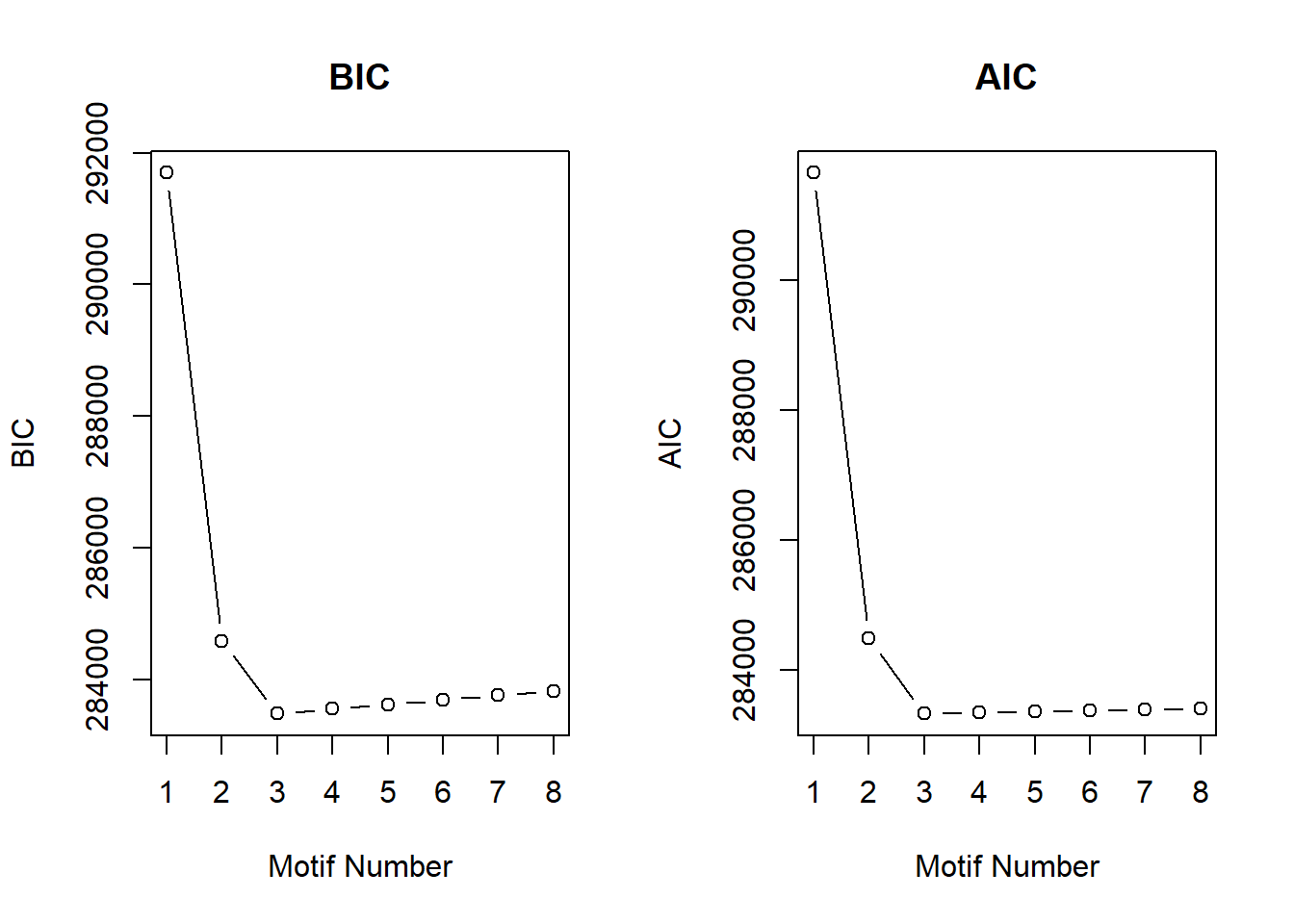

Past versions of Model1-1.png

Version	Author	Date
41cd1be	sayanpaul01	2025-02-27
ce4b325	sayanpaul01	2025-02-25

plotMotif(cormotif_0.1)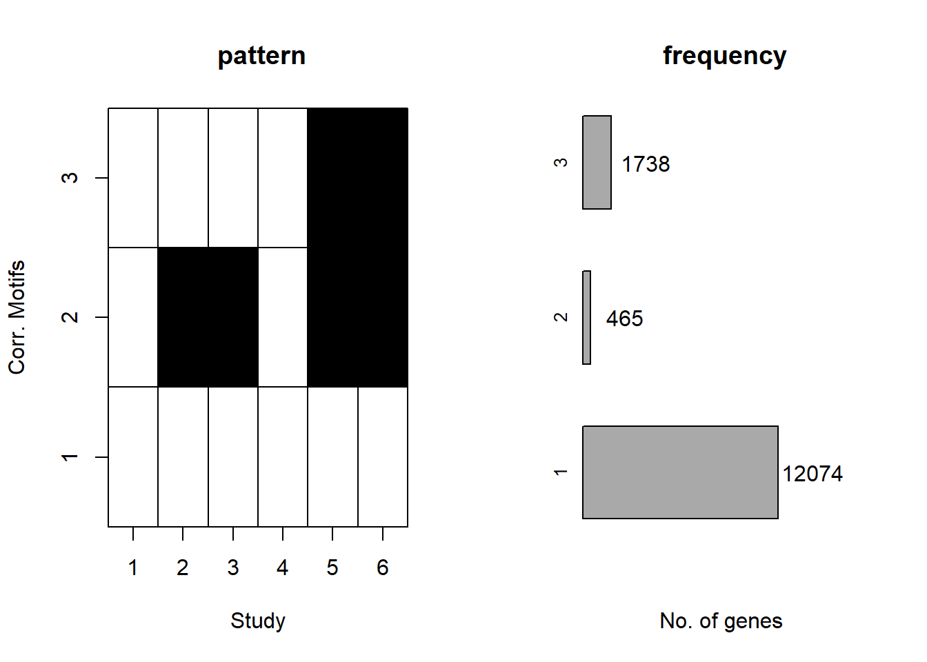

Past versions of Model1-2.png

Version	Author	Date
41cd1be	sayanpaul01	2025-02-27
ce4b325	sayanpaul01	2025-02-25

📌 Extract Gene Probabilities (0.1 Micromolar)

# Extract posterior probabilities for genes
gene_prob_tran_0.1 <- cormotif_0.1$bestmotif$p.post

rownames(gene_prob_tran_0.1) <- rownames(Corrmotif_df)

# Define gene probability groups
prob_1_0.1  <- rownames(gene_prob_tran_0.1[(gene_prob_tran_0.1[,1] <0.5 & gene_prob_tran_0.1[,2] <0.5 & gene_prob_tran_0.1[,3] <0.5 & gene_prob_tran_0.1[,4] <0.5 & gene_prob_tran_0.1[,5] < 0.5 & gene_prob_tran_0.1[,6]<0.5),])
length(prob_1_0.1)

[1] 12308

prob_2_0.1  <- rownames(gene_prob_tran_0.1[(gene_prob_tran_0.1[,1] <0.5 & gene_prob_tran_0.1[,2] >0.5 & gene_prob_tran_0.1[,3] >0.5 & gene_prob_tran_0.1[,4] <0.5 & gene_prob_tran_0.1[,5] > 0.5 & gene_prob_tran_0.1[,6]>0.5),])
length(prob_2_0.1)

[1] 415

prob_3_0.1  <- rownames(gene_prob_tran_0.1[(gene_prob_tran_0.1[,1] <0.5 & gene_prob_tran_0.1[,2] <0.5 & gene_prob_tran_0.1[,3] <0.5 & gene_prob_tran_0.1[,4] <0.5 & gene_prob_tran_0.1[,5] > 0.5 & gene_prob_tran_0.1[,6]>0.5),])
length(prob_3_0.1)

[1] 1551

📌 Distribution of Gene Clusters Identified by Corrmotif (0.1 micromolar)

# Load necessary library
library(ggplot2)

# Data
data <- data.frame(
  Category = c("Non response (0.1 µM)", "CX-DOX mid-late response (0.1 µM)", "DOX only mid-late (0.1 µM)"),
  Value = c(12308, 415, 1551)
)

# Define custom colors
custom_colors <- c("Non response (0.1 µM)" = "#FF9999",
                   "CX-DOX mid-late response (0.1 µM)" = "#66B2FF",
                   "DOX only mid-late (0.1 µM)" = "#99FF99")

# Create pie chart
ggplot(data, aes(x = "", y = Value, fill = Category)) +
  geom_bar(width = 1, stat = "identity") +
  coord_polar("y", start = 0) +
  geom_text(aes(label = Value),
            position = position_stack(vjust = 0.5),
            size = 4, color = "black") +
  labs(title = "Pie Chart (0.1 micromolar Corrmotif)", x = NULL, y = NULL) +
  theme_void() +
  scale_fill_manual(values = custom_colors)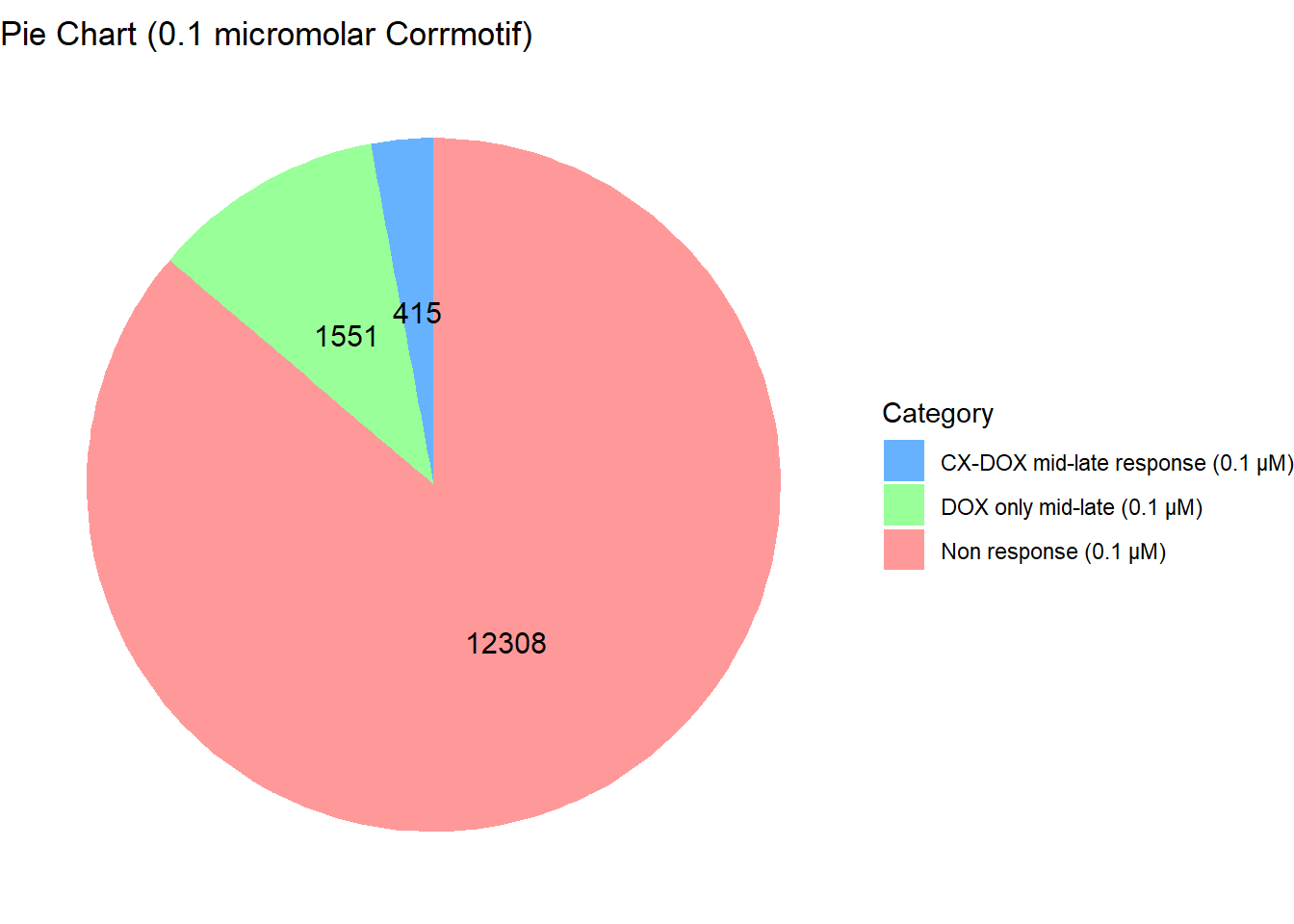

Past versions of pie-chart_0.1-1.png

Version	Author	Date
2de67e6	sayanpaul01	2025-02-27

📌 Save Corr-motif datasets for Gene Ontology analysis (0.1 Micromolar)

write.csv(data.frame(Entrez_ID = prob_1_0.1), "data/prob_1_0.1.csv", row.names = FALSE)
write.csv(data.frame(Entrez_ID = prob_2_0.1), "data/prob_2_0.1.csv", row.names = FALSE)
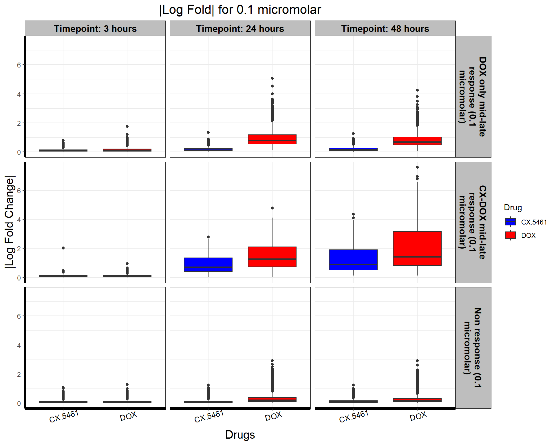
write.csv(data.frame(Entrez_ID = prob_3_0.1), "data/prob_3_0.1.csv", row.names = FALSE)

📌 0.1 Micromolar abs logFC

# Load Required Libraries
library(dplyr)
library(ggplot2)

# Load Response Groups from CSV Files
prob_1_0.1 <- as.character(read.csv("data/prob_1_0.1.csv")$Entrez_ID)
prob_2_0.1 <- as.character(read.csv("data/prob_2_0.1.csv")$Entrez_ID)
prob_3_0.1 <- as.character(read.csv("data/prob_3_0.1.csv")$Entrez_ID)

# Load Datasets (Only 0.1 Micromolar)
CX_0.1_3  <- read.csv("data/DEGs/Toptable_CX_0.1_3.csv")
CX_0.1_24 <- read.csv("data/DEGs/Toptable_CX_0.1_24.csv")
CX_0.1_48 <- read.csv("data/DEGs/Toptable_CX_0.1_48.csv")

DOX_0.1_3  <- read.csv("data/DEGs/Toptable_DOX_0.1_3.csv")
DOX_0.1_24 <- read.csv("data/DEGs/Toptable_DOX_0.1_24.csv")
DOX_0.1_48 <- read.csv("data/DEGs/Toptable_DOX_0.1_48.csv")

# Combine All 0.1 Micromolar Datasets into a Single Dataframe
all_toptables_0.1 <- bind_rows(
  CX_0.1_3  %>% mutate(Drug = "CX.5461", Timepoint = "Timepoint: 3 hours"),
  CX_0.1_24 %>% mutate(Drug = "CX.5461", Timepoint = "Timepoint: 24 hours"),
  CX_0.1_48 %>% mutate(Drug = "CX.5461", Timepoint = "Timepoint: 48 hours"),
  DOX_0.1_3  %>% mutate(Drug = "DOX", Timepoint = "Timepoint: 3 hours"),
  DOX_0.1_24 %>% mutate(Drug = "DOX", Timepoint = "Timepoint: 24 hours"),
  DOX_0.1_48 %>% mutate(Drug = "DOX", Timepoint = "Timepoint: 48 hours")
)

# Convert `Entrez_ID` to Character to Avoid `%in%` Issues
all_toptables_0.1$Entrez_ID <- as.character(all_toptables_0.1$Entrez_ID)

# Assign Response Groups with Line Breaks for Better Plotting
all_toptables_0.1 <- all_toptables_0.1 %>%
  mutate(
    Response_Group = case_when(
      Entrez_ID %in% prob_1_0.1 ~ "Non response\n(0.1 micromolar)",
      Entrez_ID %in% prob_2_0.1 ~ "CX-DOX mid-late response\n(0.1 micromolar)",
      Entrez_ID %in% prob_3_0.1 ~ "DOX only mid-late response\n(0.1 micromolar)",
      TRUE ~ NA_character_
    )
  ) %>%
  filter(!is.na(Response_Group))

# Compute Absolute logFC
all_toptables_0.1 <- all_toptables_0.1 %>%
  mutate(absFC = abs(logFC))

# Convert Factors for Proper Ordering (Reversed Order for Response Groups)
all_toptables_0.1 <- all_toptables_0.1 %>%
  mutate(
    Drug = factor(Drug, levels = c("CX.5461", "DOX")),
    Timepoint = factor(Timepoint, levels = c("Timepoint: 3 hours", "Timepoint: 24 hours", "Timepoint: 48 hours")),
    Response_Group = factor(Response_Group,
                            levels = c(
                              "DOX only mid-late response\n(0.1 micromolar)",
                              "CX-DOX mid-late response\n(0.1 micromolar)",
                              "Non response\n(0.1 micromolar)"  # Reversed Order
                            ))
  )

# **Plot the Boxplot with Faceted Labels Wrapping Correctly**
ggplot(all_toptables_0.1, aes(x = Drug, y = absFC, fill = Drug)) +
  geom_boxplot() +
  scale_fill_manual(values = c("CX.5461" = "blue", "DOX" = "red")) +  # Custom color palette
  facet_grid(Response_Group ~ Timepoint, labeller = label_wrap_gen(width = 20)) +  # Ensure Proper Wrapping
  theme_bw() +
  labs(
    x = "Drugs",
    y = "|Log Fold Change|",
    title = "|Log Fold| for 0.1 micromolar"
  ) +
  theme(
    plot.title = element_text(size = rel(1.5), hjust = 0.5),
    axis.title = element_text(size = 15, color = "black"),
    axis.line = element_line(linewidth = 1.5),
    strip.background = element_rect(fill = "gray"),  # Gray background for facet labels
    strip.text = element_text(size = 12, color = "black", face = "bold"),  # Bold styling for facet labels
    axis.text.x = element_text(size = 10, color = "black", angle = 15)
  )

Past versions of "0.1abs logFC-1.png"

Version	Author	Date
91a7ce4	sayanpaul01	2025-03-03
d9ff853	sayanpaul01	2025-03-03

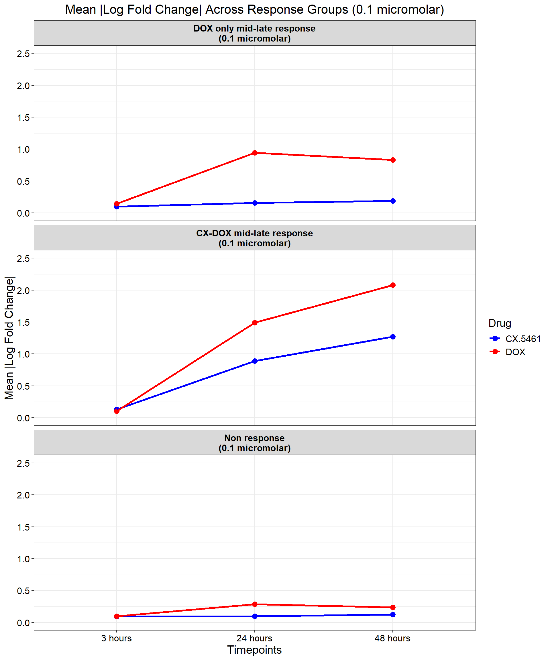
📌 0.1 Micromolar mean (Abs logFC) across timepoints

# Load Required Libraries
library(dplyr)
library(ggplot2)

# Load Response Groups from CSV Files
prob_1_0.1 <- as.character(read.csv("data/prob_1_0.1.csv")$Entrez_ID)
prob_2_0.1 <- as.character(read.csv("data/prob_2_0.1.csv")$Entrez_ID)
prob_3_0.1 <- as.character(read.csv("data/prob_3_0.1.csv")$Entrez_ID)

# Load Datasets (Only 0.1 Micromolar)
CX_0.1_3  <- read.csv("data/DEGs/Toptable_CX_0.1_3.csv")
CX_0.1_24 <- read.csv("data/DEGs/Toptable_CX_0.1_24.csv")
CX_0.1_48 <- read.csv("data/DEGs/Toptable_CX_0.1_48.csv")

DOX_0.1_3  <- read.csv("data/DEGs/Toptable_DOX_0.1_3.csv")
DOX_0.1_24 <- read.csv("data/DEGs/Toptable_DOX_0.1_24.csv")
DOX_0.1_48 <- read.csv("data/DEGs/Toptable_DOX_0.1_48.csv")

# Combine All 0.1 Micromolar Datasets into a Single Dataframe
all_toptables_0.1 <- bind_rows(
  CX_0.1_3  %>% mutate(Drug = "CX.5461", Timepoint = "3"),
  CX_0.1_24 %>% mutate(Drug = "CX.5461", Timepoint = "24"),
  CX_0.1_48 %>% mutate(Drug = "CX.5461", Timepoint = "48"),
  DOX_0.1_3  %>% mutate(Drug = "DOX", Timepoint = "3"),
  DOX_0.1_24 %>% mutate(Drug = "DOX", Timepoint = "24"),
  DOX_0.1_48 %>% mutate(Drug = "DOX", Timepoint = "48")
)

# Convert `Entrez_ID` to Character to Avoid `%in%` Issues
all_toptables_0.1$Entrez_ID <- as.character(all_toptables_0.1$Entrez_ID)

# Assign Response Groups with Line Breaks for Better Plotting
all_toptables_0.1 <- all_toptables_0.1 %>%
  mutate(
    Response_Group = case_when(
      Entrez_ID %in% prob_1_0.1 ~ "Non response\n(0.1 micromolar)",
      Entrez_ID %in% prob_2_0.1 ~ "CX-DOX mid-late response\n(0.1 micromolar)",
      Entrez_ID %in% prob_3_0.1 ~ "DOX only mid-late response\n(0.1 micromolar)",
      TRUE ~ NA_character_
    )
  ) %>%
  filter(!is.na(Response_Group))

# Compute Mean Absolute logFC for Line Plot
data_summary <- all_toptables_0.1 %>%
  mutate(abs_logFC = abs(logFC)) %>%  # Take absolute log fold change
  group_by(Response_Group, Drug, Timepoint) %>%
  dplyr::summarize(mean_abs_logFC = mean(abs_logFC, na.rm = TRUE), .groups = "drop") %>%
  as.data.frame()

# **Ensure all timepoints exist in the summary**
timepoints_full <- expand.grid(
  Response_Group = unique(all_toptables_0.1$Response_Group),
  Drug = unique(all_toptables_0.1$Drug),
  Timepoint = c("3", "24", "48")
)

# **Merge to keep missing timepoints**
data_summary <- full_join(timepoints_full, data_summary, by = c("Response_Group", "Drug", "Timepoint"))

# **Replace NA mean_abs_logFC with 0 if no genes were present**
data_summary$mean_abs_logFC[is.na(data_summary$mean_abs_logFC)] <- 0

# Convert Factors for Proper Ordering (Reversed Order for Response Groups)
data_summary <- data_summary %>%
  mutate(
    Timepoint = factor(Timepoint, levels = c("3", "24", "48"), labels = c("3 hours", "24 hours", "48 hours")),
    Response_Group = factor(Response_Group, levels = c(
      "DOX only mid-late response\n(0.1 micromolar)",
      "CX-DOX mid-late response\n(0.1 micromolar)",
      "Non response\n(0.1 micromolar)"  # Reversed Order
    ))
  )

# Define custom drug palette
drug_palette <- c("CX.5461" = "blue", "DOX" = "red")

# **Plot the Line Plot for Absolute logFC**
ggplot(data_summary, aes(x = Timepoint, y = mean_abs_logFC, group = Drug, color = Drug)) +
  geom_point(size = 3) +
  geom_line(size = 1.2) +
  scale_color_manual(values = drug_palette) +
  ylim(0, 2.5) +  # Adjust the Y-axis for better visualization
  facet_wrap(~ Response_Group, ncol = 1) +  # Facet by Response Group (Reversed Order)
  theme_bw() +
  labs(
    x = "Timepoints",
    y = "Mean |Log Fold Change|",
    title = "Mean |Log Fold Change| Across Response Groups (0.1 micromolar)",
    color = "Drug"
  ) +
  theme(
    plot.title = element_text(size = rel(1.5), hjust = 0.5),
    axis.title = element_text(size = 15, color = "black"),
    axis.text = element_text(size = 12, color = "black"),
    strip.text = element_text(size = 12, color = "black", face = "bold"),
    legend.title = element_text(size = 14),
    legend.text = element_text(size = 12)
  )

Past versions of "0.1 mean-1.png"

Version	Author	Date
91a7ce4	sayanpaul01	2025-03-03
d9ff853	sayanpaul01	2025-03-03

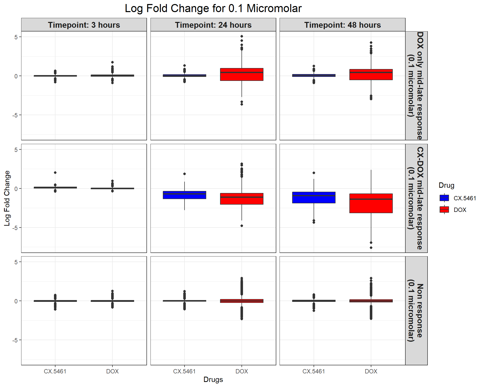
📌 0.1 Micromolar logFC

# Load required libraries
library(dplyr)
library(ggplot2)

# Load Response Groups from CSV Files
prob_1_0.1 <- as.character(read.csv("data/prob_1_0.1.csv")$Entrez_ID)
prob_2_0.1 <- as.character(read.csv("data/prob_2_0.1.csv")$Entrez_ID)
prob_3_0.1 <- as.character(read.csv("data/prob_3_0.1.csv")$Entrez_ID)

# Load Datasets (Only 0.1 Micromolar)
CX_0.1_3  <- read.csv("data/DEGs/Toptable_CX_0.1_3.csv")
CX_0.1_24 <- read.csv("data/DEGs/Toptable_CX_0.1_24.csv")
CX_0.1_48 <- read.csv("data/DEGs/Toptable_CX_0.1_48.csv")

DOX_0.1_3  <- read.csv("data/DEGs/Toptable_DOX_0.1_3.csv")
DOX_0.1_24 <- read.csv("data/DEGs/Toptable_DOX_0.1_24.csv")
DOX_0.1_48 <- read.csv("data/DEGs/Toptable_DOX_0.1_48.csv")

# Combine All 0.1 Micromolar Datasets into a Single Dataframe
all_toptables_0.1 <- bind_rows(
  CX_0.1_3  %>% mutate(Drug = "CX.5461", Timepoint = "Timepoint: 3 hours"),
  CX_0.1_24 %>% mutate(Drug = "CX.5461", Timepoint = "Timepoint: 24 hours"),
  CX_0.1_48 %>% mutate(Drug = "CX.5461", Timepoint = "Timepoint: 48 hours"),
  DOX_0.1_3  %>% mutate(Drug = "DOX", Timepoint = "Timepoint: 3 hours"),
  DOX_0.1_24 %>% mutate(Drug = "DOX", Timepoint = "Timepoint: 24 hours"),
  DOX_0.1_48 %>% mutate(Drug = "DOX", Timepoint = "Timepoint: 48 hours")
)

# Convert `Entrez_ID` to Character to Avoid `%in%` Issues
all_toptables_0.1$Entrez_ID <- as.character(all_toptables_0.1$Entrez_ID)

# Assign Response Groups with Line Breaks for Better Plotting
all_toptables_0.1 <- all_toptables_0.1 %>%
  mutate(
    Response_Group = case_when(
      Entrez_ID %in% prob_1_0.1 ~ "Non response\n(0.1 micromolar)",
      Entrez_ID %in% prob_2_0.1 ~ "CX-DOX mid-late response\n(0.1 micromolar)",
      Entrez_ID %in% prob_3_0.1 ~ "DOX only mid-late response\n(0.1 micromolar)",
      TRUE ~ NA_character_
    )
  ) %>%
  filter(!is.na(Response_Group))

# Convert factors to ensure correct ordering (Reversed Order for Response Groups)
all_toptables_0.1 <- all_toptables_0.1 %>%
  mutate(
    Timepoint = factor(Timepoint, levels = c("Timepoint: 3 hours", "Timepoint: 24 hours", "Timepoint: 48 hours")),
    Response_Group = factor(Response_Group, levels = c(
      "DOX only mid-late response\n(0.1 micromolar)",
      "CX-DOX mid-late response\n(0.1 micromolar)",
      "Non response\n(0.1 micromolar)"  # Reversed Order
    ))
  )

# **Plot the Boxplot**
ggplot(all_toptables_0.1, aes(x = Drug, y = logFC, fill = Drug)) +
  geom_boxplot() +
  scale_fill_manual(values = c("CX.5461" = "blue", "DOX" = "red")) +
  facet_grid(Response_Group ~ Timepoint) +
  theme_bw() +
  labs(x = "Drugs", y = "Log Fold Change", title = "Log Fold Change for 0.1 Micromolar") +
  theme(
    plot.title = element_text(size = rel(1.5), hjust = 0.5),
    strip.text = element_text(size = 12, face = "bold")
  )

Past versions of "0.1 logFC-1.png"

Version	Author	Date
91a7ce4	sayanpaul01	2025-03-03
d9ff853	sayanpaul01	2025-03-03

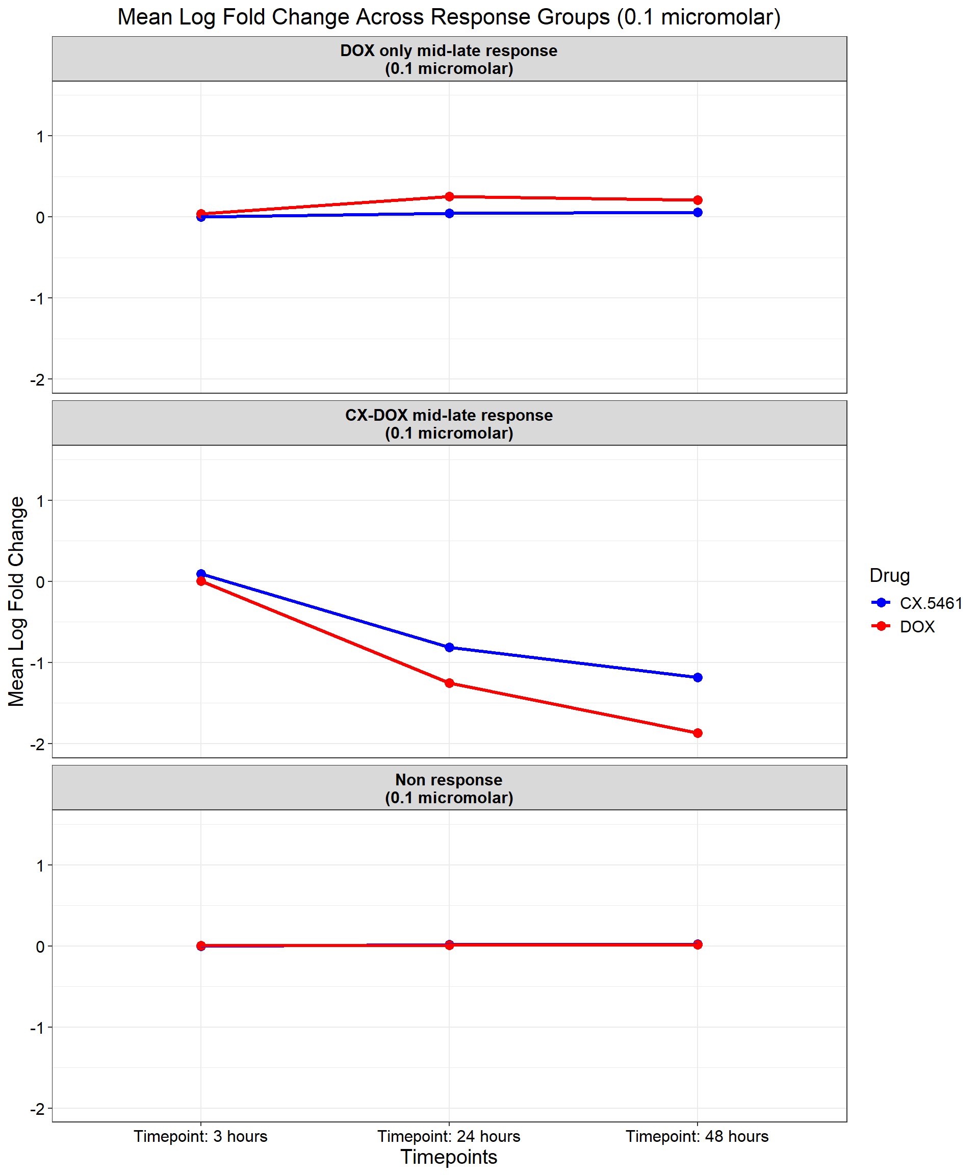
📌 0.1 Micromolar mean logFC across timepoints

# Compute Mean logFC for Line Plot
data_summary <- all_toptables_0.1 %>%
  group_by(Response_Group, Drug, Timepoint) %>%
  dplyr::summarize(mean_logFC = mean(logFC, na.rm = TRUE), .groups = "drop") %>%
  as.data.frame()

# Convert factors to ensure correct ordering (Reversed Order for Response Groups)
data_summary <- data_summary %>%
  mutate(
    Timepoint = factor(Timepoint, levels = c("Timepoint: 3 hours", "Timepoint: 24 hours", "Timepoint: 48 hours")),
    Response_Group = factor(Response_Group, levels = c(
      "DOX only mid-late response\n(0.1 micromolar)",
      "CX-DOX mid-late response\n(0.1 micromolar)",
      "Non response\n(0.1 micromolar)"  # Reversed Order
    ))
  )

# **Plot the Line Plot**
ggplot(data_summary, aes(x = Timepoint, y = mean_logFC, group = Drug, color = Drug)) +
  geom_point(size = 3) +
  geom_line(size = 1.2) +
  scale_color_manual(values = c("CX.5461" = "blue", "DOX" = "red")) +
  ylim(-2, 1.5) +  # Adjust the Y-axis for better visualization
  facet_wrap(~ Response_Group, ncol = 1) +  # Facet by Response Group (Reversed Order)
  theme_bw() +
  labs(
    x = "Timepoints",
    y = "Mean Log Fold Change",
    title = "Mean Log Fold Change Across Response Groups (0.1 micromolar)",
    color = "Drug"
  ) +
  theme(
    plot.title = element_text(size = rel(1.5), hjust = 0.5),
    axis.title = element_text(size = 15, color = "black"),
    axis.text = element_text(size = 12, color = "black"),
    strip.text = element_text(size = 12, color = "black", face = "bold"),
    legend.title = element_text(size = 14),
    legend.text = element_text(size = 12)
  )

Past versions of "0.1 mean2-1.png"

Version	Author	Date
91a7ce4	sayanpaul01	2025-03-03
d9ff853	sayanpaul01	2025-03-03

📌 Corrmotif Model 0.5 Micromolar

📌 Load Corrmotif Data

# Read the Corrmotif Results
Corrmotif <- read.csv("data/Corrmotif/CX5461.csv")
Corrmotif_df <- data.frame(Corrmotif)
rownames(Corrmotif_df) <- Corrmotif_df$Gene

# Filter for 0.5 Concentration Only
exprs.corrmotif <- as.matrix(Corrmotif_df[, grep("0.5", colnames(Corrmotif_df))])


# Read group and comparison IDs
groupid <- read.csv("data/Corrmotif/groupid.csv")
groupid_df <- data.frame(groupid[, grep("0.5", colnames(groupid))])


compid <- read.csv("data/Corrmotif/Compid.csv")
compid_df <- compid[compid$Cond1 %in% unique(as.numeric(groupid_df)) & compid$Cond2 %in% unique(as.numeric(groupid_df)), ]

📌 Corrmotif Model 0.5 Micromolar (K=1:8)

📌 Fit Corrmotif Model (K=1:8) (0.5 Micromolar)

# Fit Corrmotif Model (K = 1 to 8)
set.seed(11111)
motif.fitted_0.5 <- cormotiffit(
  exprs = exprs.corrmotif,
  groupid = groupid_df,
  compid = compid_df,
  K = 1:8,
  max.iter = 1000,
  BIC = TRUE,
  runtype = "logCPM"
)

gene_prob_0.5 <- motif.fitted_0.5$bestmotif$p.post
rownames(gene_prob_0.5) <- rownames(Corrmotif_df)
motif_prob_0.5 <- motif.fitted_0.5$bestmotif$clustlike
rownames(motif_prob_0.5) <- rownames(gene_prob_0.5)
write.csv(motif_prob_0.5,"data/cormotif_probability_genelist_0.5.csv")

📌 Plot motif (0.5 Micromolar)

cormotif_0.5 <- readRDS("data/Corrmotif/cormotif_0.5.RDS")

cormotif_0.5$bic

     K      bic
[1,] 1 352140.7
[2,] 2 346785.8
[3,] 3 344812.9
[4,] 4 344860.1
[5,] 5 344751.9
[6,] 6 344820.8
[7,] 7 344889.7
[8,] 8 344966.6

plotIC(cormotif_0.5)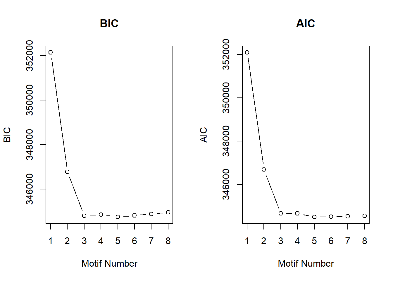

Past versions of Motif_0.5-1.png

Version	Author	Date
41cd1be	sayanpaul01	2025-02-27

plotMotif(cormotif_0.5)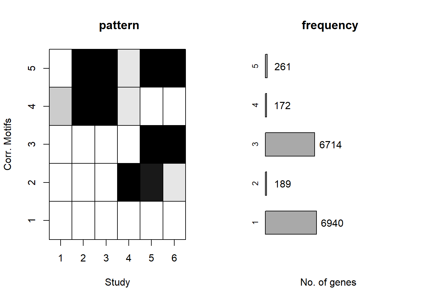

Past versions of Motif_0.5-2.png

Version	Author	Date
41cd1be	sayanpaul01	2025-02-27

📌 Extract Gene Probabilities (0.5 Micromolar)

# Extract posterior probabilities for genes
gene_prob_tran_0.5 <- cormotif_0.5$bestmotif$p.post

rownames(gene_prob_tran_0.5) <- rownames(Corrmotif_df)

# Define gene probability groups
prob_1_0.5  <- rownames(gene_prob_tran_0.5[(gene_prob_tran_0.5[,1] <0.5 & gene_prob_tran_0.5[,2] <0.5 & gene_prob_tran_0.5[,3] <0.5 & gene_prob_tran_0.5[,4] <0.5 & gene_prob_tran_0.5[,5] < 0.5 & gene_prob_tran_0.5[,6]<0.5),])
length(prob_1_0.5)

[1] 7134

prob_2_0.5  <- rownames(gene_prob_tran_0.5[(gene_prob_tran_0.5[,1] <0.5 & gene_prob_tran_0.5[,2] <0.5 & gene_prob_tran_0.5[,3] <0.5 & gene_prob_tran_0.5[,4] >0.5 & gene_prob_tran_0.5[,5] > 0.5 & gene_prob_tran_0.5[,6]>=0.02),])
length(prob_2_0.5)

[1] 179

prob_3_0.5  <- rownames(gene_prob_tran_0.5[(gene_prob_tran_0.5[,1] <0.5 & gene_prob_tran_0.5[,2] <0.5 & gene_prob_tran_0.5[,3] <0.5 & gene_prob_tran_0.5[,4] <0.5 & gene_prob_tran_0.5[,5] > 0.5 & gene_prob_tran_0.5[,6]>0.5),])
length(prob_3_0.5)

[1] 6450

prob_4_0.5  <- rownames(gene_prob_tran_0.5[(gene_prob_tran_0.5[,1] >= 0.1 & gene_prob_tran_0.5[,2] > 0.5 & gene_prob_tran_0.5[,3] > 0.5 & gene_prob_tran_0.5[,4] >= 0.02 & gene_prob_tran_0.5[,5] < 0.5 & gene_prob_tran_0.5[,6] < 0.5),]) 

length(prob_4_0.5)

[1] 142

prob_5_0.5  <- rownames(gene_prob_tran_0.5[(gene_prob_tran_0.5[,1] <0.5 & gene_prob_tran_0.5[,2] >0.5 & gene_prob_tran_0.5[,3] >0.5 & gene_prob_tran_0.5[,4] >=0.02 & gene_prob_tran_0.5[,4] <0.5 & gene_prob_tran_0.5[,5] > 0.5 & gene_prob_tran_0.5[,6]>0.5),])
length(prob_5_0.5)

[1] 221

📌 Distribution of Gene Clusters Identified by Corrmotif (0.5 micromolar)

# Load necessary library
library(ggplot2)

# Data
data <- data.frame(
  Category = c("Non response (0.5)", "DOX-specific response (0.5 µM)", "DOX only mid-late response (0.5 µM)", "CX + DOX (early) response (0.5 µM)", "DOX + CX (mid-late) response (0.5 µM)"),
  Value = c(7134,179,6450,142,221)
)

# Add values to category names (to be displayed in the legend)
data$Category <- paste0(data$Category, " (", data$Value, ")")

# Define custom colors with updated category names
custom_colors <- setNames(
  c("#FF9999", "#FF66CC", "#66B2FF", "#99FF99", "#FFD700"),
  data$Category  # Ensures color names match updated categories
)

# Create pie chart without number labels inside
ggplot(data, aes(x = "", y = Value, fill = Category)) +
  geom_bar(width = 1, stat = "identity") +
  coord_polar("y", start = 0) +
  labs(title = "Pie Chart (0.5 micromolar Corrmotif)", x = NULL, y = NULL) +
  theme_void() +
  scale_fill_manual(values = custom_colors)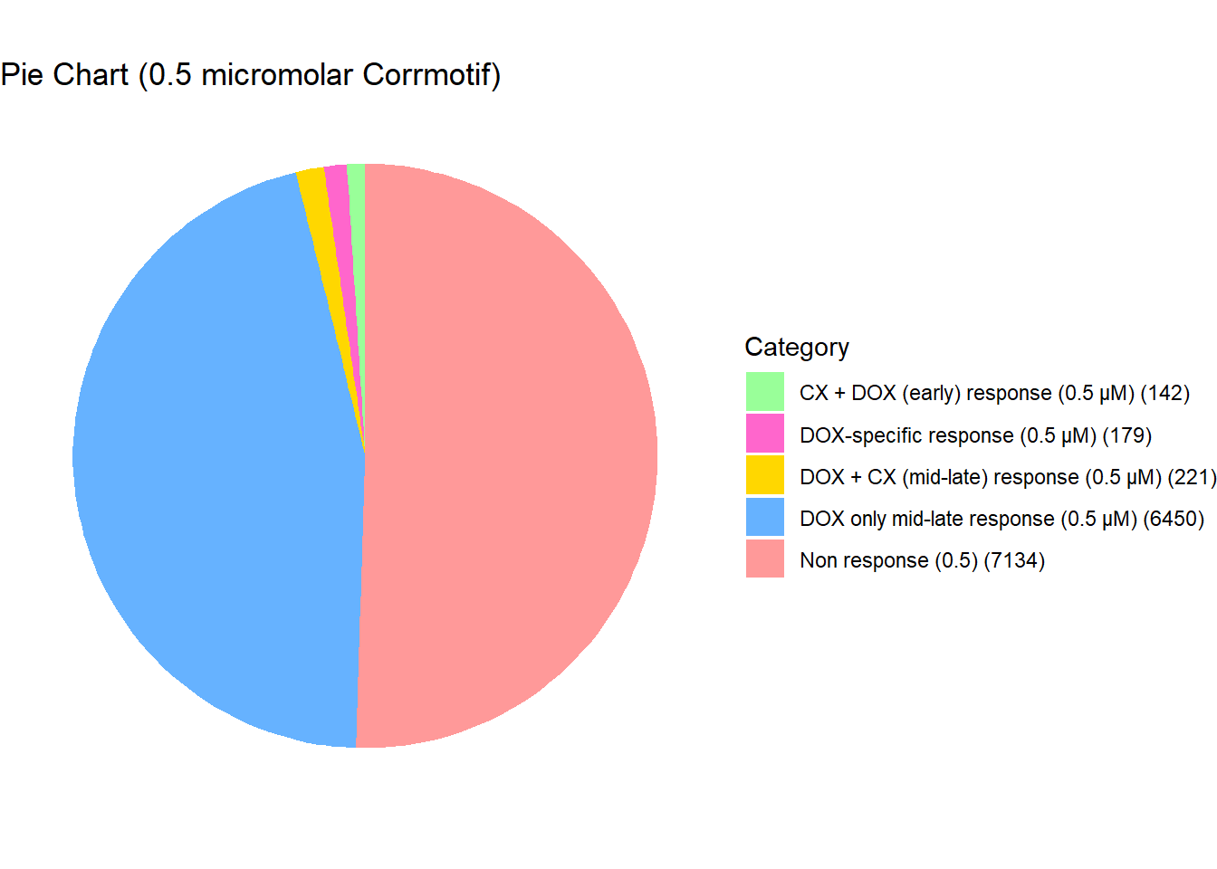

Past versions of pie-chart_0.5-1.png

Version	Author	Date
d9ff853	sayanpaul01	2025-03-03
2de67e6	sayanpaul01	2025-02-27

📌 Combined pie charts for concentrations

# Load necessary libraries
library(ggplot2)
library(dplyr)

# Data for 0.1 µM
data_0.1 <- data.frame(
  Category = c("Non response", "CX-DOX mid-late response", "DOX only mid-late"),
  Value = c(12308, 415, 1551),
  Concentration = "0.1 µM"
)

# Data for 0.5 µM
data_0.5 <- data.frame(
  Category = c("Non response", "DOX specific response", "DOX only mid-late response", 
               "CX + DOX (early) response", "DOX + CX (mid-late) response"),
  Value = c(7134, 179, 6450, 142, 221),
  Concentration = "0.5 µM"
)

# Combine both datasets
combined_data <- bind_rows(data_0.1, data_0.5)

# Add values to category names (for legend only)
combined_data$Category_Legend <- paste0(combined_data$Category, " (", combined_data$Value, ")")

# Define custom colors for updated categories
custom_colors <- c(
  "Non response (12308)" = "#FF9999",
  "CX-DOX mid-late response (415)" = "#66B2FF",
  "DOX only mid-late (1551)" = "#99FF99",
  "Non response (7134)" = "#FF9999",
  "DOX specific response (179)" = "#FF66CC",
  "DOX only mid-late response (6450)" = "#99FF99",
  "CX + DOX (early) response (142)" = "#FFD700",
  "DOX + CX (mid-late) response (221)" = "#8A2BE2"
)

# Ensure categories appear in a specific order
combined_data$Category_Legend <- factor(combined_data$Category_Legend, levels = names(custom_colors))

# Create faceted pie charts without numbers inside the slices
pie_chart <- ggplot(combined_data, aes(x = "", y = Value, fill = Category_Legend)) +
  geom_bar(width = 1, stat = "identity") +
  coord_polar("y", start = 0) +
  facet_wrap(~ Concentration) +  # Facet by concentration (side-by-side)
  labs(title = "Corrmotif Pie Charts for 0.1 µM and 0.5 µM", x = NULL, y = NULL, fill = "Category") +
  theme_void() +
  theme(
    panel.border = element_rect(color = "black", fill = NA, linewidth = 1.5),  # Adds box around facets
    strip.background = element_rect(fill = "white", color = "black", linewidth = 1),  # Box for facet titles
    strip.text = element_text(size = 12, face = "bold", color = "black"),
    legend.title = element_text(size = 12, face = "bold"),  # Bold legend title
    legend.text = element_text(size = 10)  # Adjust legend text size
  ) +
  scale_fill_manual(values = custom_colors)

# Display the plot
print(pie_chart)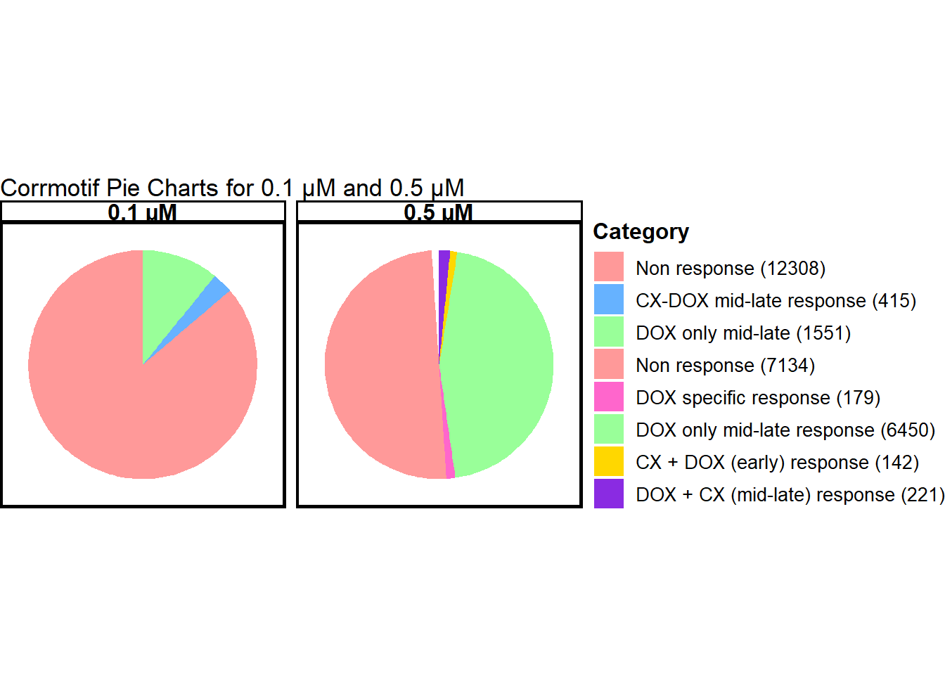

Past versions of pie-chart_comb-1.png

Version	Author	Date
ef3a951	sayanpaul01	2025-03-09

📌 Save Corr-motif datasets for Gene Ontology analysis (0.5 Micromolar)

write.csv(data.frame(Entrez_ID = prob_1_0.5), "data/prob_1_0.5.csv", row.names = FALSE)
write.csv(data.frame(Entrez_ID = prob_2_0.5), "data/prob_2_0.5.csv", row.names = FALSE)
write.csv(data.frame(Entrez_ID = prob_3_0.5), "data/prob_3_0.5.csv", row.names = FALSE)
write.csv(data.frame(Entrez_ID = prob_4_0.5), "data/prob_4_0.5.csv", row.names = FALSE)
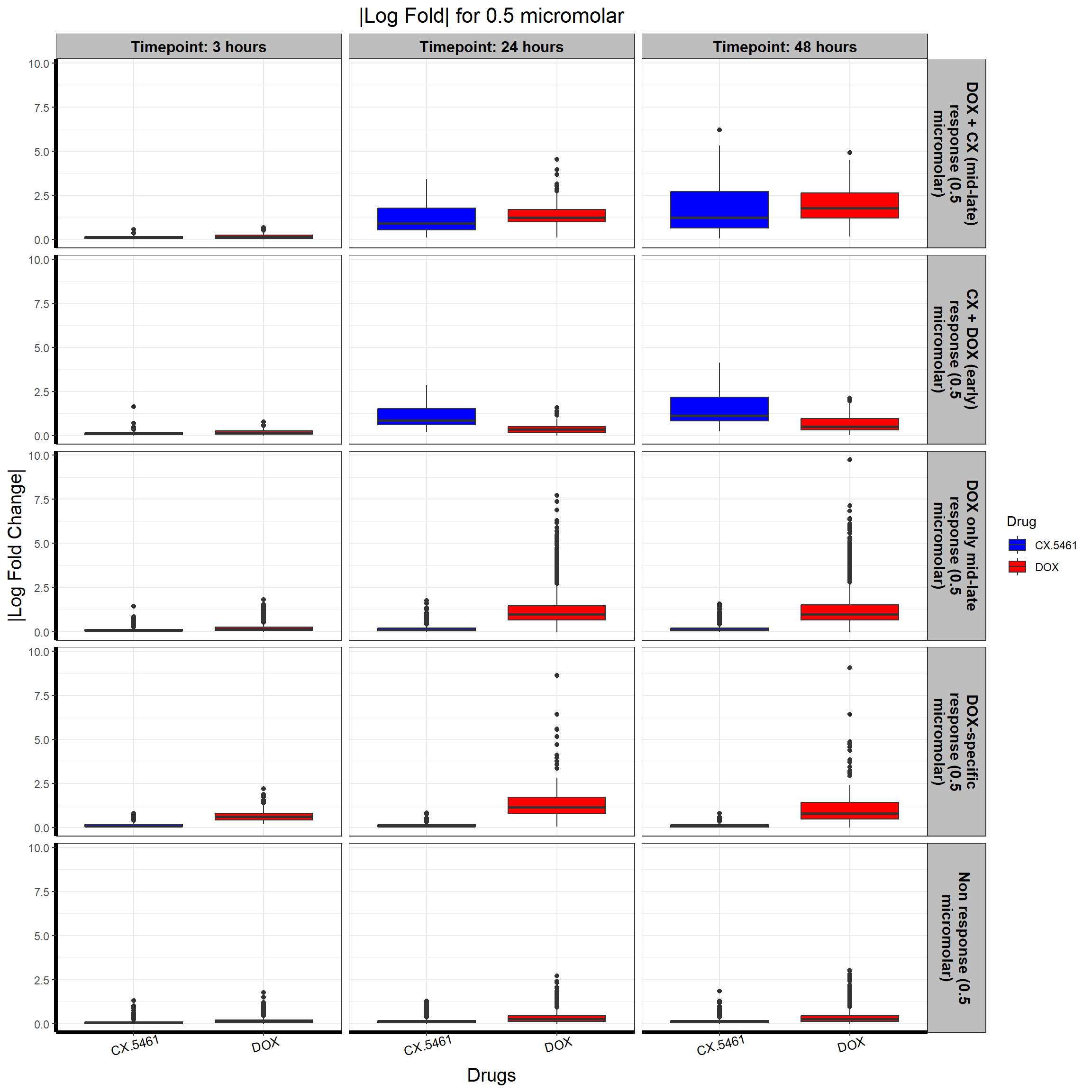
write.csv(data.frame(Entrez_ID = prob_5_0.5), "data/prob_5_0.5.csv", row.names = FALSE)

📌 0.5 Micromolar abs logFC

# Load Response Groups from CSV Files
prob_1_0.5 <- as.character(read.csv("data/prob_1_0.5.csv")$Entrez_ID)
prob_2_0.5 <- as.character(read.csv("data/prob_2_0.5.csv")$Entrez_ID)
prob_3_0.5 <- as.character(read.csv("data/prob_3_0.5.csv")$Entrez_ID)
prob_4_0.5 <- as.character(read.csv("data/prob_4_0.5.csv")$Entrez_ID)
prob_5_0.5 <- as.character(read.csv("data/prob_5_0.5.csv")$Entrez_ID)

# Load Datasets (Only 0.5 Micromolar)
CX_0.5_3  <- read.csv("data/DEGs/Toptable_CX_0.5_3.csv")
CX_0.5_24 <- read.csv("data/DEGs/Toptable_CX_0.5_24.csv")
CX_0.5_48 <- read.csv("data/DEGs/Toptable_CX_0.5_48.csv")

DOX_0.5_3  <- read.csv("data/DEGs/Toptable_DOX_0.5_3.csv")
DOX_0.5_24 <- read.csv("data/DEGs/Toptable_DOX_0.5_24.csv")
DOX_0.5_48 <- read.csv("data/DEGs/Toptable_DOX_0.5_48.csv")

# Convert datasets to DataFrames
Toptable_CX_0.5_3_df  <- data.frame(CX_0.5_3)
Toptable_CX_0.5_24_df <- data.frame(CX_0.5_24)
Toptable_CX_0.5_48_df <- data.frame(CX_0.5_48)

Toptable_DOX_0.5_3_df  <- data.frame(DOX_0.5_3)
Toptable_DOX_0.5_24_df <- data.frame(DOX_0.5_24)
Toptable_DOX_0.5_48_df <- data.frame(DOX_0.5_48)

# Combine All 0.5 Micromolar Datasets into a Single Dataframe
all_toptables_0.5 <- bind_rows(
  Toptable_CX_0.5_3_df  %>% mutate(Drug = "CX.5461", Timepoint = "3"),
  Toptable_CX_0.5_24_df %>% mutate(Drug = "CX.5461", Timepoint = "24"),
  Toptable_CX_0.5_48_df %>% mutate(Drug = "CX.5461", Timepoint = "48"),
  Toptable_DOX_0.5_3_df  %>% mutate(Drug = "DOX", Timepoint = "3"),
  Toptable_DOX_0.5_24_df %>% mutate(Drug = "DOX", Timepoint = "24"),
  Toptable_DOX_0.5_48_df %>% mutate(Drug = "DOX", Timepoint = "48")
)

# Convert `Entrez_ID` to Character to Avoid `%in%` Issues
all_toptables_0.5$Entrez_ID <- as.character(all_toptables_0.5$Entrez_ID)

# Assign Response Groups with Line Breaks for Better Plotting
all_toptables_0.5 <- all_toptables_0.5 %>%
  mutate(
    Response_Group = case_when(
      Entrez_ID %in% prob_1_0.5 ~ "Non response\n(0.5 micromolar)",
      Entrez_ID %in% prob_2_0.5 ~ "DOX-specific response\n(0.5 micromolar)",
      Entrez_ID %in% prob_3_0.5 ~ "DOX only mid-late response\n(0.5 micromolar)",
      Entrez_ID %in% prob_4_0.5 ~ "CX + DOX (early) response\n(0.5 micromolar)",
      Entrez_ID %in% prob_5_0.5 ~ "DOX + CX (mid-late) response\n(0.5 micromolar)",
      TRUE ~ NA_character_
    )
  )

# Remove NA Values (Genes Not in Response Groups)
all_toptables_0.5 <- all_toptables_0.5 %>% filter(!is.na(Response_Group))

# Compute Absolute logFC
all_toptables_0.5 <- all_toptables_0.5 %>%
  mutate(absFC = abs(logFC))

# Convert Factors for Proper Ordering (Reversed Order for Response Groups)
all_toptables_0.5 <- all_toptables_0.5 %>%
  mutate(
    Drug = factor(Drug, levels = c("CX.5461", "DOX")),
    Timepoint = factor(Timepoint, levels = c("3", "24", "48"),
                       labels = c("Timepoint: 3 hours", "Timepoint: 24 hours", "Timepoint: 48 hours")),
    Response_Group = factor(Response_Group,
                            levels = c("DOX + CX (mid-late) response\n(0.5 micromolar)",
                                       "CX + DOX (early) response\n(0.5 micromolar)",
                                       "DOX only mid-late response\n(0.5 micromolar)",
                                       "DOX-specific response\n(0.5 micromolar)",
                                       "Non response\n(0.5 micromolar)")) # Reversed Order
  )

# **Plot the Boxplot with Faceted Labels Wrapping Correctly**
ggplot(all_toptables_0.5, aes(x = Drug, y = absFC, fill = Drug)) +
  geom_boxplot() +
  scale_fill_manual(values = c("CX.5461" = "blue", "DOX" = "red")) +  # Custom color palette
  facet_grid(Response_Group ~ Timepoint, labeller = label_wrap_gen(width = 20)) +  # Ensure Proper Wrapping
  theme_bw() +
  labs(
    x = "Drugs",
    y = "|Log Fold Change|",
    title = "|Log Fold| for 0.5 micromolar"
  ) +
  theme(
    plot.title = element_text(size = rel(1.5), hjust = 0.5),
    axis.title = element_text(size = 15, color = "black"),
    axis.line = element_line(linewidth = 1.5),
    strip.background = element_rect(fill = "gray"),  # Gray background for facet labels
    strip.text = element_text(size = 12, color = "black", face = "bold"),  # Bold styling for facet labels
    axis.text.x = element_text(size = 10, color = "black", angle = 15)
  )

Past versions of "0.5abs logFC-1.png"

Version	Author	Date
91a7ce4	sayanpaul01	2025-03-03
d9ff853	sayanpaul01	2025-03-03

📌 0.5 Micromolar mean (Abs logFC) across timepoints

# Load required libraries
library(dplyr)
library(ggplot2)

# Load Response Groups from CSV Files
prob_1_0.5 <- as.character(read.csv("data/prob_1_0.5.csv")$Entrez_ID)
prob_2_0.5 <- as.character(read.csv("data/prob_2_0.5.csv")$Entrez_ID)
prob_3_0.5 <- as.character(read.csv("data/prob_3_0.5.csv")$Entrez_ID)
prob_4_0.5 <- as.character(read.csv("data/prob_4_0.5.csv")$Entrez_ID)
prob_5_0.5 <- as.character(read.csv("data/prob_5_0.5.csv")$Entrez_ID)

# Load Datasets (Only 0.5 Micromolar)
CX_0.5_3  <- read.csv("data/DEGs/Toptable_CX_0.5_3.csv")
CX_0.5_24 <- read.csv("data/DEGs/Toptable_CX_0.5_24.csv")
CX_0.5_48 <- read.csv("data/DEGs/Toptable_CX_0.5_48.csv")

DOX_0.5_3  <- read.csv("data/DEGs/Toptable_DOX_0.5_3.csv")
DOX_0.5_24 <- read.csv("data/DEGs/Toptable_DOX_0.5_24.csv")
DOX_0.5_48 <- read.csv("data/DEGs/Toptable_DOX_0.5_48.csv")

# Combine All 0.5 Micromolar Datasets into a Single Dataframe
all_toptables_0.5 <- bind_rows(
  CX_0.5_3  %>% mutate(Drug = "CX.5461", Timepoint = "3"),
  CX_0.5_24 %>% mutate(Drug = "CX.5461", Timepoint = "24"),
  CX_0.5_48 %>% mutate(Drug = "CX.5461", Timepoint = "48"),
  DOX_0.5_3  %>% mutate(Drug = "DOX", Timepoint = "3"),
  DOX_0.5_24 %>% mutate(Drug = "DOX", Timepoint = "24"),
  DOX_0.5_48 %>% mutate(Drug = "DOX", Timepoint = "48")
)

# Convert `Entrez_ID` to Character to Avoid `%in%` Issues
all_toptables_0.5$Entrez_ID <- as.character(all_toptables_0.5$Entrez_ID)

# Assign Response Groups with Line Breaks for Better Plotting
all_toptables_0.5 <- all_toptables_0.5 %>%
  mutate(
    Response_Group = case_when(
      Entrez_ID %in% prob_1_0.5 ~ "Non response\n(0.5 micromolar)",
      Entrez_ID %in% prob_2_0.5 ~ "DOX-specific response\n(0.5 micromolar)",
      Entrez_ID %in% prob_3_0.5 ~ "DOX only mid-late response\n(0.5 micromolar)",
      Entrez_ID %in% prob_4_0.5 ~ "CX + DOX (early) response\n(0.5 micromolar)",
      Entrez_ID %in% prob_5_0.5 ~ "DOX + CX (mid-late) response\n(0.5 micromolar)",
      TRUE ~ NA_character_
    )
  ) %>%
  filter(!is.na(Response_Group))  # Remove NA values

# Compute Mean Absolute logFC for Line Plot
data_summary <- all_toptables_0.5 %>%
  mutate(abs_logFC = abs(logFC)) %>%
  group_by(Response_Group, Drug, Timepoint) %>%
  dplyr::summarize(mean_abs_logFC = mean(abs_logFC, na.rm = TRUE), .groups = "drop") %>%
  as.data.frame()

# **Ensure all timepoints exist in the summary**
timepoints_full <- expand.grid(
  Response_Group = unique(all_toptables_0.5$Response_Group),
  Drug = unique(all_toptables_0.5$Drug),
  Timepoint = c("3", "24", "48")
)

# **Merge to keep missing timepoints**
data_summary <- full_join(timepoints_full, data_summary, by = c("Response_Group", "Drug", "Timepoint"))

# **Replace NA mean_abs_logFC with 0 if no genes were present**
data_summary$mean_abs_logFC[is.na(data_summary$mean_abs_logFC)] <- 0

# Convert Factors for Proper Ordering (Reversed Order for Response Groups)
data_summary <- data_summary %>%
  mutate(
    Timepoint = factor(Timepoint, levels = c("3", "24", "48"), labels = c("3 hours", "24 hours", "48 hours")),
    Response_Group = factor(Response_Group, levels = c(
      "DOX + CX (mid-late) response\n(0.5 micromolar)",
                                       "CX + DOX (early) response\n(0.5 micromolar)",
                                       "DOX only mid-late response\n(0.5 micromolar)",
                                       "DOX-specific response\n(0.5 micromolar)",
                                       "Non response\n(0.5 micromolar)"  # Reversed order
    ))
  )

# Define custom drug palette
drug_palette <- c("CX.5461" = "blue", "DOX" = "red")

# **Plot the Line Plot for Mean Absolute logFC**
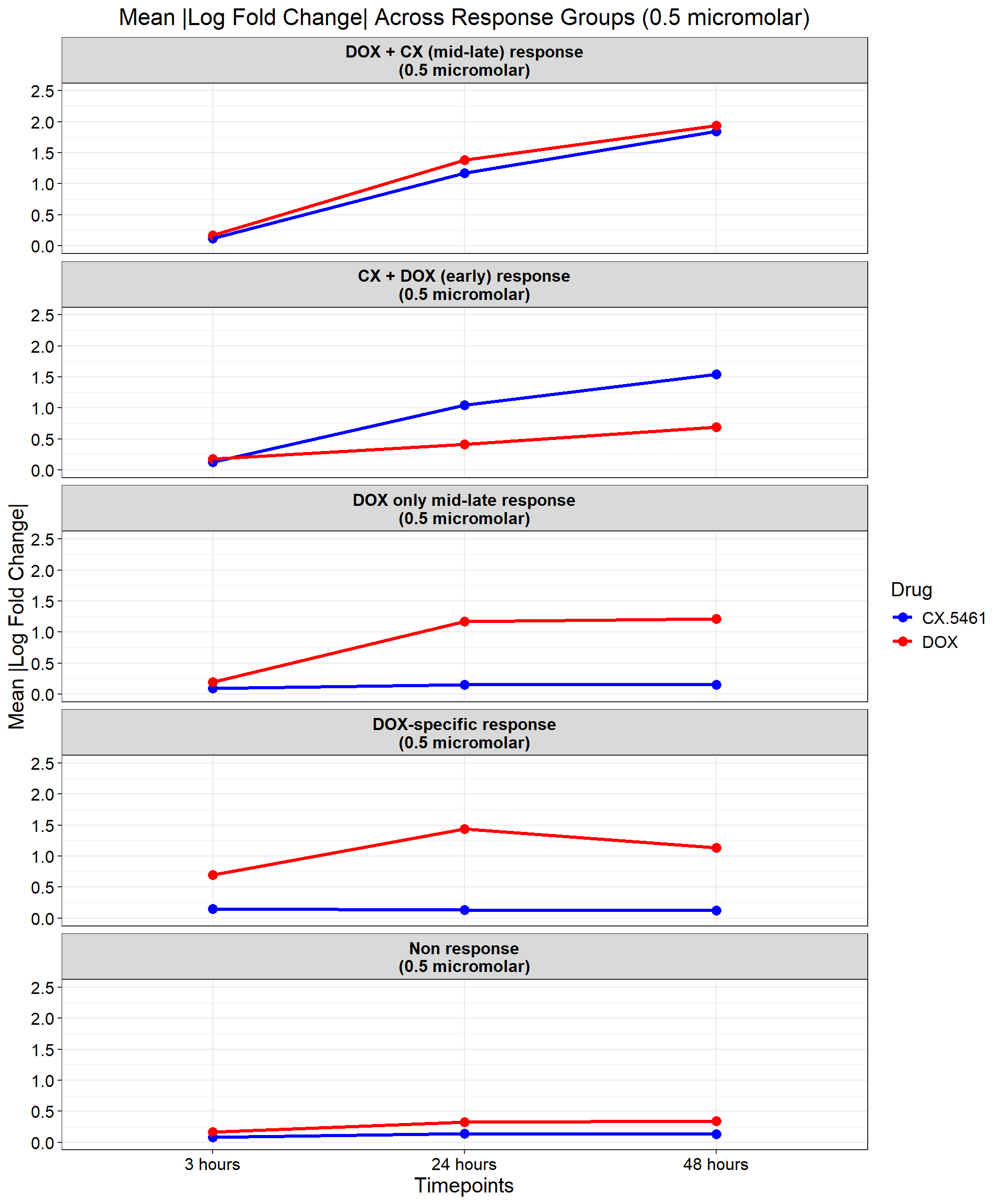
ggplot(data_summary, aes(x = Timepoint, y = mean_abs_logFC, group = Drug, color = Drug)) +
  geom_point(size = 3) +
  geom_line(size = 1.2) +
  scale_color_manual(values = drug_palette) +
  ylim(0, 2.5) +  # Adjust the Y-axis for better visualization
  facet_wrap(~ Response_Group, ncol = 1) +  # Facet by Response Group (Reversed Order)
  theme_bw() +
  labs(
    x = "Timepoints",
    y = "Mean |Log Fold Change|",
    title = "Mean |Log Fold Change| Across Response Groups (0.5 micromolar)",
    color = "Drug"
  ) +
  theme(
    plot.title = element_text(size = rel(1.5), hjust = 0.5),
    axis.title = element_text(size = 15, color = "black"),
    axis.text = element_text(size = 12, color = "black"),
    strip.text = element_text(size = 12, color = "black", face = "bold"),
    legend.title = element_text(size = 14),
    legend.text = element_text(size = 12)
  )

Past versions of "0.5 mean-1.png"

Version	Author	Date
91a7ce4	sayanpaul01	2025-03-03
d9ff853	sayanpaul01	2025-03-03

📌 0.5 Micromolar logFC

# Load required libraries
library(dplyr)
library(ggplot2)

# Load Response Groups from CSV Files
prob_1_0.5 <- as.character(read.csv("data/prob_1_0.5.csv")$Entrez_ID)
prob_2_0.5 <- as.character(read.csv("data/prob_2_0.5.csv")$Entrez_ID)
prob_3_0.5 <- as.character(read.csv("data/prob_3_0.5.csv")$Entrez_ID)
prob_4_0.5 <- as.character(read.csv("data/prob_4_0.5.csv")$Entrez_ID)
prob_5_0.5 <- as.character(read.csv("data/prob_5_0.5.csv")$Entrez_ID)

# Load Datasets (Only 0.5 Micromolar)
CX_0.5_3  <- read.csv("data/DEGs/Toptable_CX_0.5_3.csv")
CX_0.5_24 <- read.csv("data/DEGs/Toptable_CX_0.5_24.csv")
CX_0.5_48 <- read.csv("data/DEGs/Toptable_CX_0.5_48.csv")

DOX_0.5_3  <- read.csv("data/DEGs/Toptable_DOX_0.5_3.csv")
DOX_0.5_24 <- read.csv("data/DEGs/Toptable_DOX_0.5_24.csv")
DOX_0.5_48 <- read.csv("data/DEGs/Toptable_DOX_0.5_48.csv")

# Combine All 0.5 Micromolar Datasets into a Single Dataframe
all_toptables_0.5 <- bind_rows(
  CX_0.5_3  %>% mutate(Drug = "CX.5461", Timepoint = "Timepoint: 3 hours"),
  CX_0.5_24 %>% mutate(Drug = "CX.5461", Timepoint = "Timepoint: 24 hours"),
  CX_0.5_48 %>% mutate(Drug = "CX.5461", Timepoint = "Timepoint: 48 hours"),
  DOX_0.5_3  %>% mutate(Drug = "DOX", Timepoint = "Timepoint: 3 hours"),
  DOX_0.5_24 %>% mutate(Drug = "DOX", Timepoint = "Timepoint: 24 hours"),
  DOX_0.5_48 %>% mutate(Drug = "DOX", Timepoint = "Timepoint: 48 hours")
)

# Convert `Entrez_ID` to Character to Avoid `%in%` Issues
all_toptables_0.5$Entrez_ID <- as.character(all_toptables_0.5$Entrez_ID)

# Assign Response Groups
all_toptables_0.5 <- all_toptables_0.5 %>%
  mutate(
    Response_Group = case_when(
      Entrez_ID %in% prob_1_0.5 ~ "Non response\n(0.5 micromolar)",
      Entrez_ID %in% prob_2_0.5 ~ "DOX-specific response\n(0.5 micromolar)",
      Entrez_ID %in% prob_3_0.5 ~ "DOX only mid-late response\n(0.5 micromolar)",
      Entrez_ID %in% prob_4_0.5 ~ "CX + DOX (early) response\n(0.5 micromolar)",
      Entrez_ID %in% prob_5_0.5 ~ "DOX + CX (mid-late) response\n(0.5 micromolar)",
      TRUE ~ NA_character_
    )
  ) %>%
  filter(!is.na(Response_Group))

# Convert factors to ensure correct ordering (Reversed Order for Response Groups)
all_toptables_0.5 <- all_toptables_0.5 %>%
  mutate(
    Timepoint = factor(Timepoint, levels = c("Timepoint: 3 hours", "Timepoint: 24 hours", "Timepoint: 48 hours")),
    Response_Group = factor(Response_Group, levels = c(
      "DOX + CX (mid-late) response\n(0.5 micromolar)",
                                       "CX + DOX (early) response\n(0.5 micromolar)",
                                       "DOX only mid-late response\n(0.5 micromolar)",
                                       "DOX-specific response\n(0.5 micromolar)",
                                       "Non response\n(0.5 micromolar)"  # Reversed Order
    ))
  )

# **Plot the Boxplot**
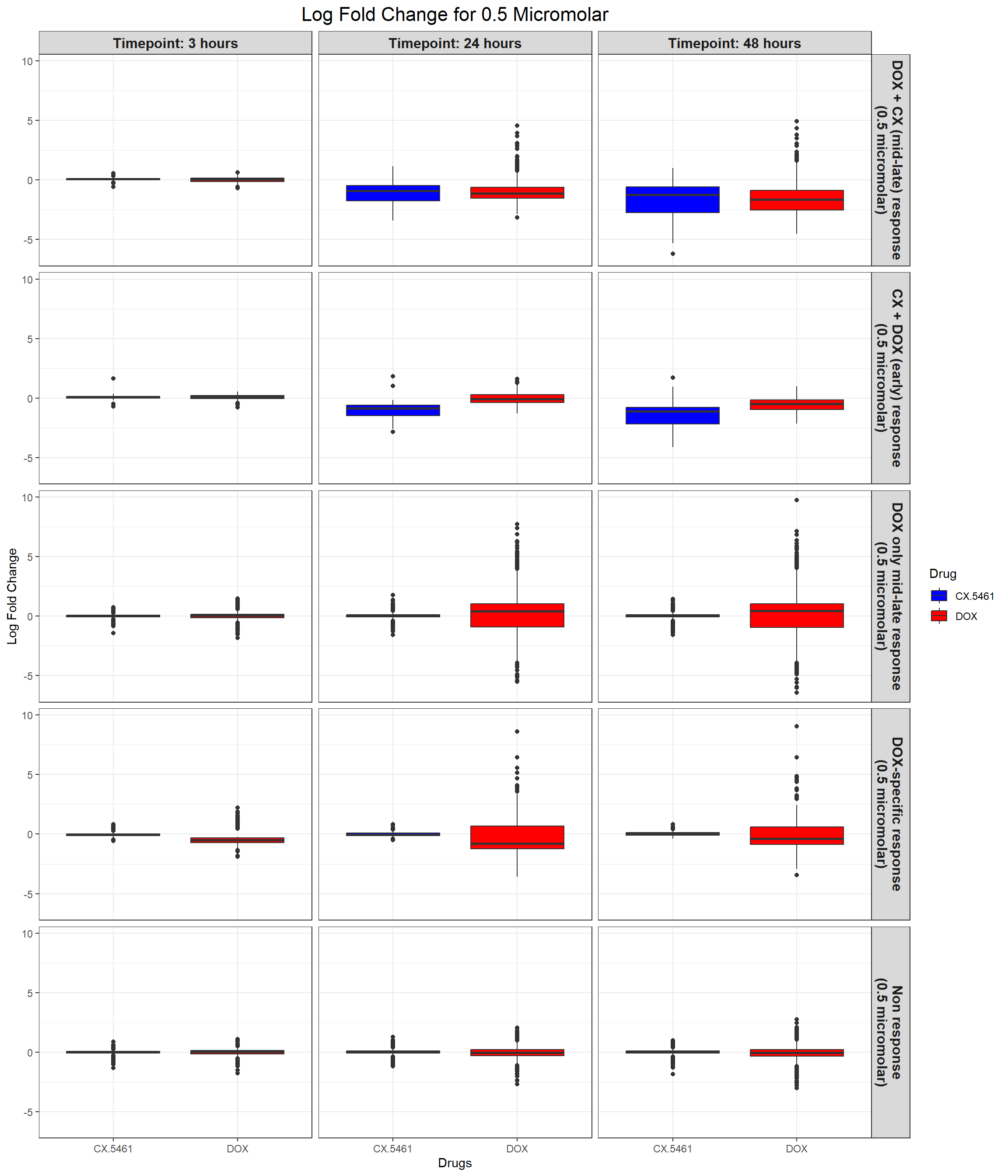
ggplot(all_toptables_0.5, aes(x = Drug, y = logFC, fill = Drug)) +
  geom_boxplot() +
  scale_fill_manual(values = c("CX.5461" = "blue", "DOX" = "red")) +
  facet_grid(Response_Group ~ Timepoint) +
  theme_bw() +
  labs(x = "Drugs", y = "Log Fold Change", title = "Log Fold Change for 0.5 Micromolar") +
  theme(
    plot.title = element_text(size = rel(1.5), hjust = 0.5),
    strip.text = element_text(size = 12, face = "bold")
  )

Past versions of 0.5logFC-1.png

Version	Author	Date
91a7ce4	sayanpaul01	2025-03-03
d9ff853	sayanpaul01	2025-03-03

📌 0.5 Micromolar mean logFC across timepoints

# Load Required Libraries
library(dplyr)
library(ggplot2)

# Load Response Groups from CSV Files
prob_1_0.5 <- as.character(read.csv("data/prob_1_0.5.csv")$Entrez_ID)
prob_2_0.5 <- as.character(read.csv("data/prob_2_0.5.csv")$Entrez_ID)
prob_3_0.5 <- as.character(read.csv("data/prob_3_0.5.csv")$Entrez_ID)
prob_4_0.5 <- as.character(read.csv("data/prob_4_0.5.csv")$Entrez_ID)
prob_5_0.5 <- as.character(read.csv("data/prob_5_0.5.csv")$Entrez_ID)

# Load Datasets (Only 0.5 Micromolar)
CX_0.5_3  <- read.csv("data/DEGs/Toptable_CX_0.5_3.csv")
CX_0.5_24 <- read.csv("data/DEGs/Toptable_CX_0.5_24.csv")
CX_0.5_48 <- read.csv("data/DEGs/Toptable_CX_0.5_48.csv")

DOX_0.5_3  <- read.csv("data/DEGs/Toptable_DOX_0.5_3.csv")
DOX_0.5_24 <- read.csv("data/DEGs/Toptable_DOX_0.5_24.csv")
DOX_0.5_48 <- read.csv("data/DEGs/Toptable_DOX_0.5_48.csv")

# Combine All 0.5 Micromolar Datasets into a Single Dataframe
all_toptables_0.5 <- bind_rows(
  CX_0.5_3  %>% mutate(Drug = "CX.5461", Timepoint = "Timepoint: 3 hours"),
  CX_0.5_24 %>% mutate(Drug = "CX.5461", Timepoint = "Timepoint: 24 hours"),
  CX_0.5_48 %>% mutate(Drug = "CX.5461", Timepoint = "Timepoint: 48 hours"),
  DOX_0.5_3  %>% mutate(Drug = "DOX", Timepoint = "Timepoint: 3 hours"),
  DOX_0.5_24 %>% mutate(Drug = "DOX", Timepoint = "Timepoint: 24 hours"),
  DOX_0.5_48 %>% mutate(Drug = "DOX", Timepoint = "Timepoint: 48 hours")
)

# Convert `Entrez_ID` to Character to Avoid `%in%` Issues
all_toptables_0.5$Entrez_ID <- as.character(all_toptables_0.5$Entrez_ID)

# Assign Response Groups with Line Breaks for Better Plotting
all_toptables_0.5 <- all_toptables_0.5 %>%
  mutate(
    Response_Group = case_when(
      Entrez_ID %in% prob_1_0.5 ~ "Non response\n(0.5 micromolar)",
      Entrez_ID %in% prob_2_0.5 ~ "DOX-specific response\n(0.5 micromolar)",
      Entrez_ID %in% prob_3_0.5 ~ "DOX only mid-late response\n(0.5 micromolar)",
      Entrez_ID %in% prob_4_0.5 ~ "CX + DOX (early) response\n(0.5 micromolar)",
      Entrez_ID %in% prob_5_0.5 ~ "DOX + CX (mid-late) response\n(0.5 micromolar)",
      TRUE ~ NA_character_
    )
  ) %>%
  filter(!is.na(Response_Group))

# Compute Mean logFC for Line Plot
data_summary_0.5 <- all_toptables_0.5 %>%
  group_by(Response_Group, Drug, Timepoint) %>%
  dplyr::summarize(mean_logFC = mean(logFC, na.rm = TRUE), .groups = "drop") %>%
  as.data.frame()

# **Ensure all timepoints exist in the summary**
timepoints_full <- expand.grid(
  Response_Group = unique(all_toptables_0.5$Response_Group),
  Drug = unique(all_toptables_0.5$Drug),
  Timepoint = c("Timepoint: 3 hours", "Timepoint: 24 hours", "Timepoint: 48 hours")
)

# **Merge to keep missing timepoints**
data_summary_0.5 <- full_join(timepoints_full, data_summary_0.5, by = c("Response_Group", "Drug", "Timepoint"))

# **Replace NA mean_logFC with 0 if no genes were present**
data_summary_0.5$mean_logFC[is.na(data_summary_0.5$mean_logFC)] <- 0

# Convert Factors for Proper Ordering (Reversed Order for Response Groups)
data_summary_0.5 <- data_summary_0.5 %>%
  mutate(
    Timepoint = factor(Timepoint, levels = c("Timepoint: 3 hours", "Timepoint: 24 hours", "Timepoint: 48 hours")),
    Response_Group = factor(Response_Group, levels = c(
      "DOX + CX (mid-late) response\n(0.5 micromolar)",
                                       "CX + DOX (early) response\n(0.5 micromolar)",
                                       "DOX only mid-late response\n(0.5 micromolar)",
                                       "DOX-specific response\n(0.5 micromolar)",
                                       "Non response\n(0.5 micromolar)"  # Reversed Order
    ))
  )

# Define custom drug palette
drug_palette <- c("CX.5461" = "blue", "DOX" = "red")

# **Plot the Line Plot for Mean logFC**
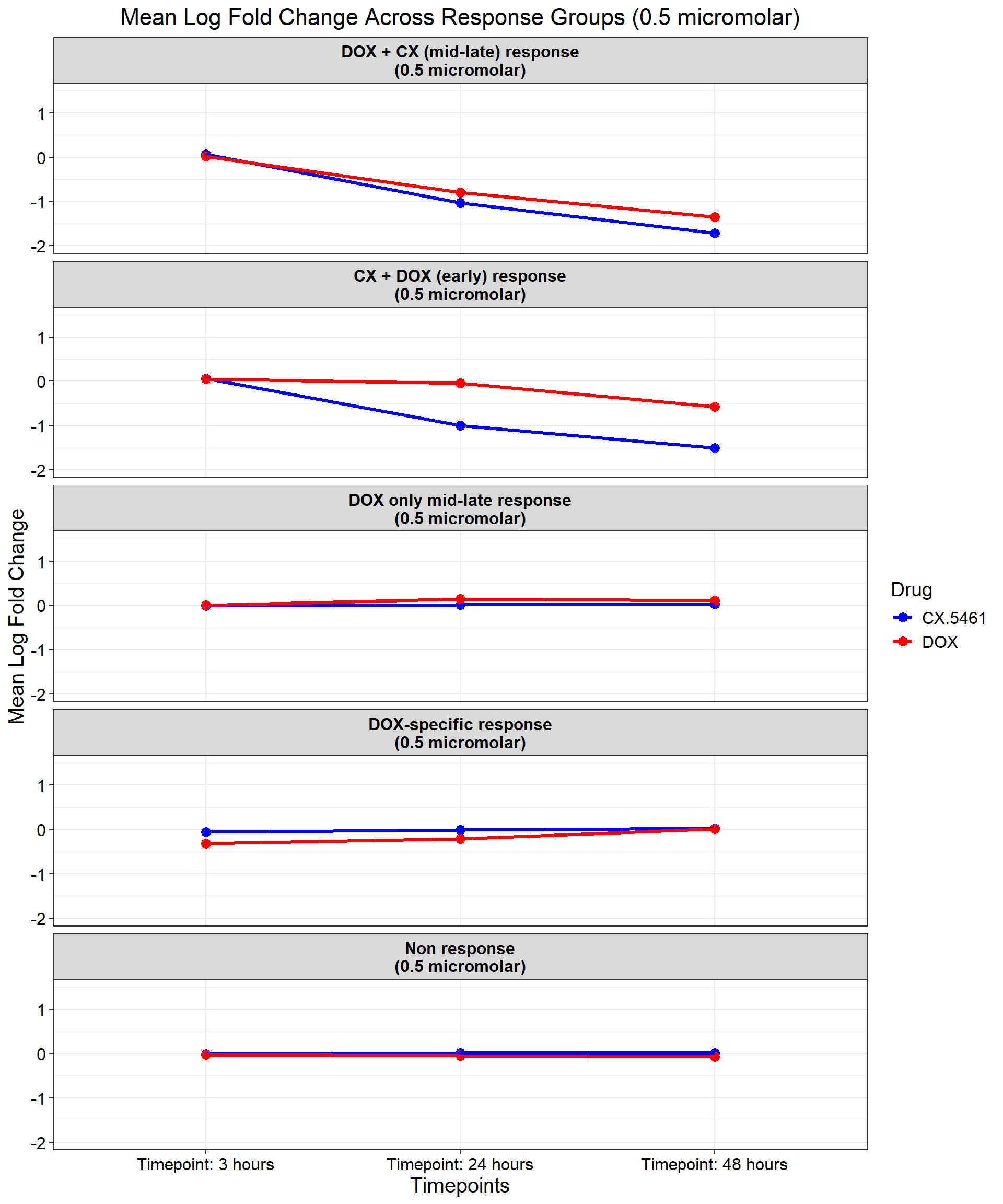
ggplot(data_summary_0.5, aes(x = Timepoint, y = mean_logFC, group = Drug, color = Drug)) +
  geom_point(size = 3) +
  geom_line(size = 1.2) +
  scale_color_manual(values = drug_palette) +
  ylim(-2, 1.5) +  # Adjust the Y-axis for better visualization
  facet_wrap(~ Response_Group, ncol = 1) +  # Facet by Response Group (Reversed Order)
  theme_bw() +
  labs(
    x = "Timepoints",
    y = "Mean Log Fold Change",
    title = "Mean Log Fold Change Across Response Groups (0.5 micromolar)",
    color = "Drug"
  ) +
  theme(
    plot.title = element_text(size = rel(1.5), hjust = 0.5),
    axis.title = element_text(size = 15, color = "black"),
    axis.text = element_text(size = 12, color = "black"),
    strip.text = element_text(size = 12, color = "black", face = "bold"),
    legend.title = element_text(size = 14),
    legend.text = element_text(size = 12)
  )

Past versions of "0.5 mean2-1.png"

Version	Author	Date
91a7ce4	sayanpaul01	2025-03-03
d9ff853	sayanpaul01	2025-03-03

📌 Proportion of DNA Damage Repair Genes (0.1 micromolar)

# Load necessary libraries
library(dplyr)
library(ggplot2)
library(tidyr)

Warning: package 'tidyr' was built under R version 4.3.3

library(org.Hs.eg.db)

Warning: package 'AnnotationDbi' was built under R version 4.3.2

Warning: package 'IRanges' was built under R version 4.3.1

Warning: package 'S4Vectors' was built under R version 4.3.1

# **🔹 Read DNA Damage Repair Gene List**
DNA_damage <- read.csv("data/DNA_Damage.csv", stringsAsFactors = FALSE)

# Convert gene symbols to Entrez IDs
DNA_damage <- DNA_damage %>%
  mutate(Entrez_ID = mapIds(org.Hs.eg.db,
                            keys = DNA_damage$Symbol,
                            column = "ENTREZID",
                            keytype = "SYMBOL",
                            multiVals = "first"))

DNA_damage_genes <- na.omit(DNA_damage$Entrez_ID)

# **🔹 Load Corrmotif Groups for 0.1 Concentration**
prob_groups_0.1 <- list(
  "Non Response (0.1)" = read.csv("data/prob_1_0.1.csv")$Entrez_ID,
   "CX_DOX mid-late (0.1)" = read.csv("data/prob_2_0.1.csv")$Entrez_ID,
  "DOX only mid-late (0.1)"= read.csv("data/prob_3_0.1.csv")$Entrez_ID
)

# **🔹 Create Dataframe for Corrmotif Groups**
corrmotif_df_0.1 <- bind_rows(
  lapply(prob_groups_0.1, function(ids) {
    data.frame(Entrez_ID = ids)
  }),
  .id = "Response_Group"
)

# **🔹 Match Entrez_IDs with DNA Damage Repair Genes**
corrmotif_df_0.1 <- corrmotif_df_0.1 %>%
  mutate(DNA_Damage = ifelse(Entrez_ID %in% DNA_damage_genes, "Yes", "No"))

# **🔹 Count DNA Damage Repair Genes in Each Response Group**
proportion_data <- corrmotif_df_0.1 %>%
  group_by(Response_Group, DNA_Damage) %>%
  summarise(Count = n(), .groups = "drop") %>%
  group_by(Response_Group) %>%
  mutate(Percentage = (Count / sum(Count)) * 100)

# **🔹 Ensure "Yes" is at the Bottom and "No" at the Top**
proportion_data$DNA_Damage <- factor(proportion_data$DNA_Damage, levels = c("Yes", "No"))

# **🔹 Set Order of Response Groups for X-axis**
response_order <- c("Non Response (0.1)", "CX_DOX mid-late (0.1)","DOX only mid-late (0.1)")
proportion_data$Response_Group <- factor(proportion_data$Response_Group, levels = response_order)

# **🔹 Perform Chi-Square Tests for "DOX only mid-late (0.1)" and "CX_DOX mid-late (0.1)" vs "Non Response (0.1)"**
non_response_counts <- proportion_data %>%
  filter(Response_Group == "Non Response (0.1)") %>%
  dplyr::select(DNA_Damage, Count) %>%
  {setNames(.$Count, .$DNA_Damage)}  # Convert to named vector

chi_results <- proportion_data %>%
  filter(Response_Group %in% c("CX_DOX mid-late (0.1)","DOX only mid-late (0.1)")) %>%
  group_by(Response_Group) %>%
  summarise(
    p_value = {
      group_counts <- Count[DNA_Damage %in% c("Yes", "No")]
      if (!"Yes" %in% DNA_Damage) group_counts <- c(group_counts, 0)
      if (!"No" %in% DNA_Damage) group_counts <- c(0, group_counts)

      contingency_table <- matrix(c(
        group_counts[1], group_counts[2],
        non_response_counts["Yes"], non_response_counts["No"]
      ), nrow = 2, byrow = TRUE)

      # Perform chi-square test if all values are valid
      if (all(contingency_table >= 0 & is.finite(contingency_table))) {
        chisq.test(contingency_table)$p.value
      } else {
        NA
      }
    },
    .groups = "drop"
  ) %>%
  mutate(Significance = ifelse(!is.na(p_value) & p_value < 0.05, "*", ""))

# **🔹 Merge Chi-Square Results into Proportion Data**
proportion_data <- proportion_data %>%
  left_join(chi_results %>% dplyr::select(Response_Group, Significance), by = "Response_Group")

# **🔹 Set Star Position Uniform Across Groups at 105%**
star_positions <- data.frame(
  Response_Group = c("CX_DOX mid-late (0.1)", "DOX only mid-late (0.1)"),
  y_pos = 105,  # Fixed at 105% of Y-axis
  Significance = chi_results$Significance
)

# **🔹 Generate Proportion Plot with Chi-Square Stars**
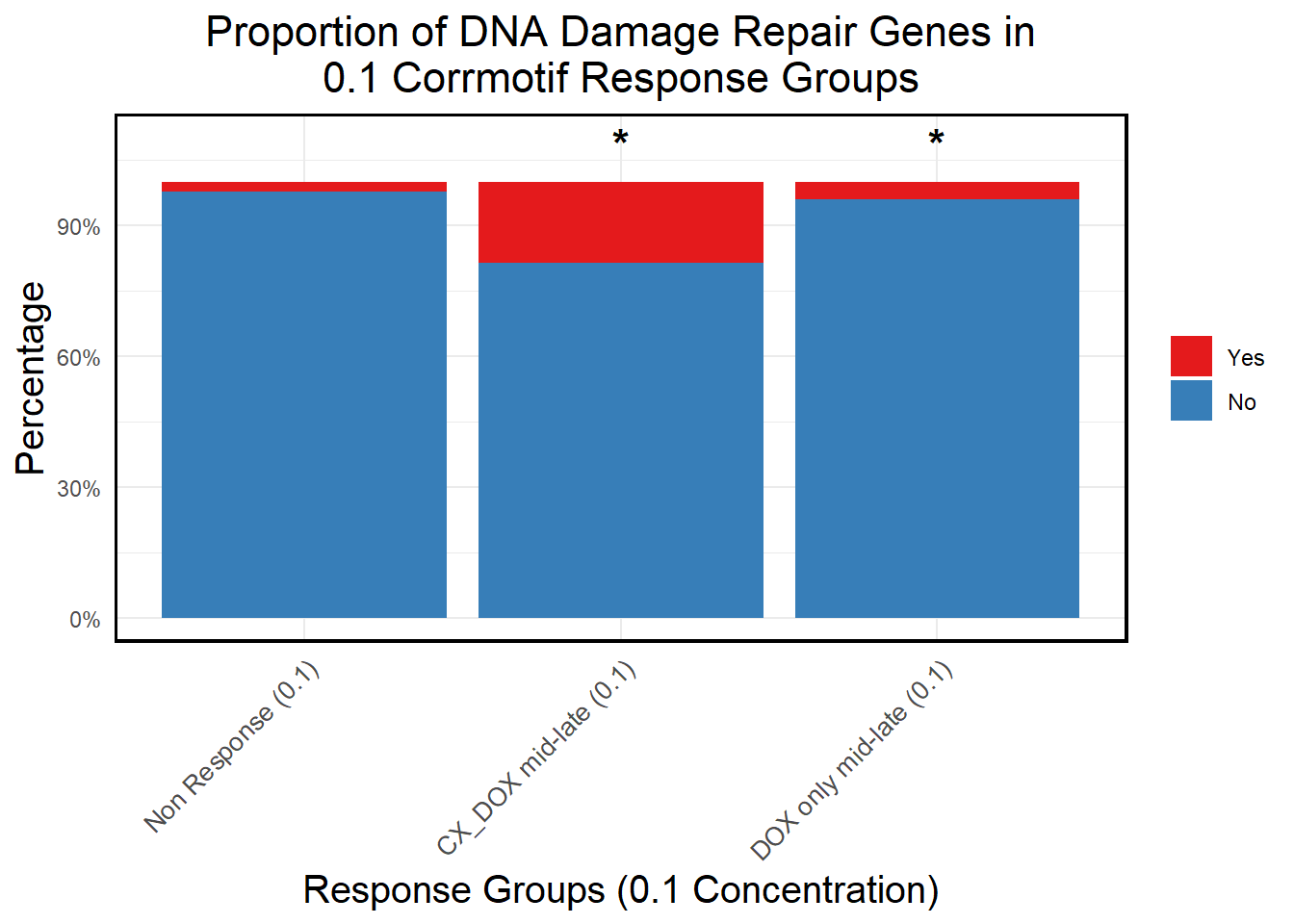
ggplot(proportion_data, aes(x = Response_Group, y = Percentage, fill = DNA_Damage)) +
  geom_bar(stat = "identity", position = "stack") +  # Stacked bars
  geom_text(
    data = star_positions,
    aes(x = Response_Group, y = y_pos, label = Significance),  # Place stars at fixed 105%
    inherit.aes = FALSE,
    size = 6, color = "black", fontface = "bold", vjust = 0  # Keeps stars aligned
  ) +
  scale_y_continuous(labels = scales::percent_format(scale = 1), limits = c(0, 110)) +  # Fixed Y-axis to 100%
  scale_fill_manual(values = c("Yes" = "#e41a1c", "No" = "#377eb8")) +  # Yes (Red), No (Blue)
  labs(
    title = "Proportion of DNA Damage Repair Genes in\n0.1 Corrmotif Response Groups",
    x = "Response Groups (0.1 Concentration)",
    y = "Percentage",
    fill = "DNA Damage Repair"
  ) +
  theme_minimal() +
  theme(
    plot.title = element_text(size = rel(1.5), hjust = 0.5),
    axis.title = element_text(size = 15, color = "black"),
    axis.text.x = element_text(size = 10, angle = 45, hjust = 1),
    legend.title = element_blank(),
    panel.border = element_rect(color = "black", fill = NA, linewidth = 1.2),
    strip.background = element_blank(),
    strip.text = element_text(size = 12, face = "bold")
  )

Past versions of "prop DNA-1.png"

Version	Author	Date
81247f6	sayanpaul01	2025-03-06
96d0db1	sayanpaul01	2025-03-05

📌 Proportion of DNA Damage Repair Genes (0.5 micromolar)

# Load necessary libraries
library(dplyr)
library(ggplot2)
library(tidyr)
library(org.Hs.eg.db)

# **🔹 Read DNA Damage Repair Gene List**
DNA_damage <- read.csv("data/DNA_Damage.csv", stringsAsFactors = FALSE)

# Convert gene symbols to Entrez IDs
DNA_damage <- DNA_damage %>%
  mutate(Entrez_ID = mapIds(org.Hs.eg.db,
                            keys = DNA_damage$Symbol,
                            column = "ENTREZID",
                            keytype = "SYMBOL",
                            multiVals = "first"))

DNA_damage_genes <- na.omit(DNA_damage$Entrez_ID)

# **🔹 Load Corrmotif Groups for 0.5 Concentration**
prob_groups_0.5 <- list(
  "Non Response (0.5)" = read.csv("data/prob_1_0.5.csv")$Entrez_ID,
  "DOX-specific response (0.5)" = read.csv("data/prob_2_0.5.csv")$Entrez_ID,
  "DOX only mid-late response (0.5)" = read.csv("data/prob_3_0.5.csv")$Entrez_ID,
  "CX DOX (early) response (0.5)" = read.csv("data/prob_4_0.5.csv")$Entrez_ID,
  "DOX + CX (mid-late) response (0.5)" = read.csv("data/prob_5_0.5.csv")$Entrez_ID
)

# **🔹 Create Dataframe for Corrmotif Groups**
corrmotif_df_0.5 <- bind_rows(
  lapply(prob_groups_0.5, function(ids) {
    data.frame(Entrez_ID = ids)
  }),
  .id = "Response_Group"
)

# **🔹 Match Entrez_IDs with DNA Damage Repair Genes**
corrmotif_df_0.5 <- corrmotif_df_0.5 %>%
  mutate(DNA_Damage = ifelse(Entrez_ID %in% DNA_damage_genes, "Yes", "No"))

# **🔹 Count DNA Damage Repair Genes in Each Response Group**
proportion_data <- corrmotif_df_0.5 %>%
  group_by(Response_Group, DNA_Damage) %>%
  summarise(Count = n(), .groups = "drop") %>%
  group_by(Response_Group) %>%
  mutate(Percentage = (Count / sum(Count)) * 100)

# **🔹 Ensure "Yes" is at the Bottom and "No" at the Top**
proportion_data$DNA_Damage <- factor(proportion_data$DNA_Damage, levels = c("Yes", "No"))

# **🔹 Set Order of Response Groups for X-axis**
response_order <- c("Non Response (0.5)", "DOX-specific response (0.5)", "DOX only mid-late response (0.5)", 
                    "CX DOX (early) response (0.5)", "DOX + CX (mid-late) response (0.5)")
proportion_data$Response_Group <- factor(proportion_data$Response_Group, levels = response_order)

# **🔹 Perform Chi-Square Tests for Each Response Group vs Non-Response**
non_response_counts <- proportion_data %>%
  filter(Response_Group == "Non Response (0.5)") %>%
  dplyr::select(DNA_Damage, Count) %>%
  {setNames(.$Count, .$DNA_Damage)}  # Convert to named vector

# **Comparing Each Group Against "Non Response (0.5)"**
chi_results <- proportion_data %>%
  filter(Response_Group %in% c("DOX-specific response (0.5)", "DOX only mid-late response (0.5)", 
                               "CX DOX (early) response (0.5)", "DOX + CX (mid-late) response (0.5)")) %>%
  group_by(Response_Group) %>%
  summarise(
    p_value = {
      group_counts <- Count[DNA_Damage %in% c("Yes", "No")]
      if (!"Yes" %in% DNA_Damage) group_counts <- c(group_counts, 0)
      if (!"No" %in% DNA_Damage) group_counts <- c(0, group_counts)

      contingency_table <- matrix(c(
        group_counts[1], group_counts[2],  # Response group counts
        non_response_counts["Yes"], non_response_counts["No"]  # Non-response counts
      ), nrow = 2, byrow = TRUE)

      # Perform chi-square test if all values are valid
      if (all(contingency_table >= 0 & is.finite(contingency_table))) {
        chisq.test(contingency_table)$p.value
      } else {
        NA
      }
    },
    .groups = "drop"
  ) %>%
  mutate(Significance = ifelse(!is.na(p_value) & p_value < 0.05, "*", ""))

# **🔹 Merge Chi-Square Results into Proportion Data**
proportion_data <- proportion_data %>%
  left_join(chi_results %>% dplyr::select(Response_Group, Significance), by = "Response_Group")

# **🔹 Set Star Position Uniform Across Groups at 105%**
star_positions <- data.frame(
  Response_Group = c("DOX-specific response (0.5)", "DOX only mid-late response (0.5)", 
                     "CX DOX (early) response (0.5)", "DOX + CX (mid-late) response (0.5)"),
  y_pos = 105,  # Fixed at 105% of Y-axis
  Significance = chi_results$Significance
)

# **🔹 Generate Proportion Plot with Chi-Square Stars**
ggplot(proportion_data, aes(x = Response_Group, y = Percentage, fill = DNA_Damage)) +
  geom_bar(stat = "identity", position = "stack") +  # Stacked bars
  geom_text(
    data = star_positions,
    aes(x = Response_Group, y = y_pos, label = Significance),  # Place stars at fixed 105%
    inherit.aes = FALSE,
    size = 6, color = "black", fontface = "bold", vjust = 0  # Keeps stars aligned
  ) +
  scale_y_continuous(labels = scales::percent_format(scale = 1), limits = c(0, 110)) +  # **Y-axis now limited to 110% for visibility**
  scale_fill_manual(values = c("Yes" = "#e41a1c", "No" = "#377eb8")) +  # Yes (Red), No (Blue)
  labs(
    title = "Proportion of DNA Damage Repair Genes in\n0.5 Corrmotif Response Groups",
    x = "Response Groups (0.5 Concentration)",
    y = "Percentage",
    fill = "DNA Damage Repair Genes"
  ) +
  theme_minimal() +
  theme(
    plot.title = element_text(size = rel(1.5), hjust = 0.5),
    axis.title = element_text(size = 15, color = "black"),
    axis.text.x = element_text(size = 10, angle = 45, hjust = 1),
    legend.title = element_blank(),
    panel.border = element_rect(color = "black", fill = NA, linewidth = 1.2),
    strip.background = element_blank(),
    strip.text = element_text(size = 12, face = "bold")
  )

Past versions of "prop DNA 0.5-1.png"

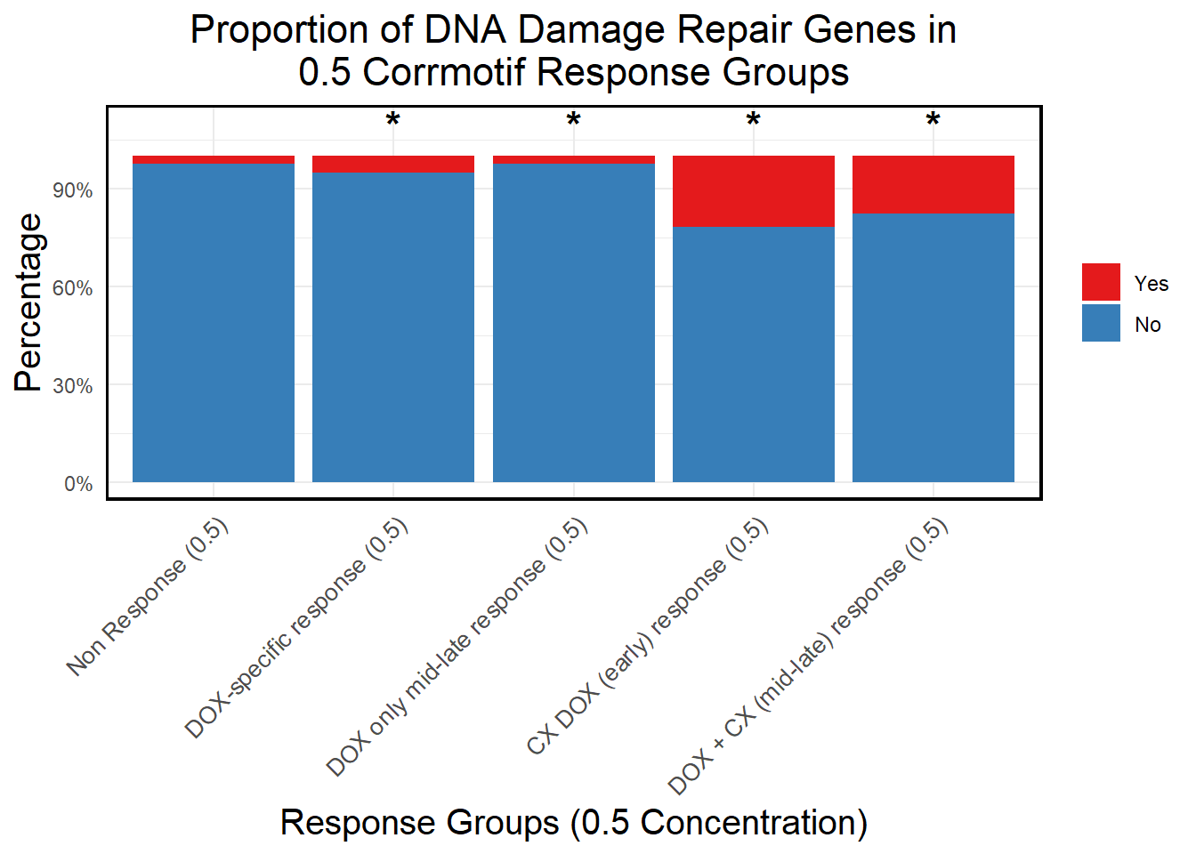
Version	Author	Date
96d0db1	sayanpaul01	2025-03-05

📌 Proportion of P53 target Genes Genes (0.1 micromolar)

# Load necessary libraries
library(dplyr)
library(ggplot2)
library(tidyr)
library(org.Hs.eg.db)

# **🔹 Read P53 Target Gene List**
P53_Target <- read.csv("data/P53_Target.csv", stringsAsFactors = FALSE)

# Convert gene symbols to Entrez IDs
P53_Target <- P53_Target %>%
  mutate(Entrez_ID = mapIds(org.Hs.eg.db,
                            keys = P53_Target$Symbol,
                            column = "ENTREZID",
                            keytype = "SYMBOL",
                            multiVals = "first"))

P53_Target_genes <- na.omit(P53_Target$Entrez_ID)

# **🔹 Load Corrmotif Groups for 0.1 Concentration**
prob_groups_0.1 <- list(
  "Non Response (0.1)" = read.csv("data/prob_1_0.1.csv")$Entrez_ID,
  "CX_DOX mid-late (0.1)" = read.csv("data/prob_2_0.1.csv")$Entrez_ID,
 "DOX only mid-late (0.1)"= read.csv("data/prob_3_0.1.csv")$Entrez_ID
)

# **🔹 Create Dataframe for Corrmotif Groups**
corrmotif_df_0.1 <- bind_rows(
  lapply(prob_groups_0.1, function(ids) {
    data.frame(Entrez_ID = ids)
  }),
  .id = "Response_Group"
)

# **🔹 Match Entrez_IDs with P53 Target Genes**
corrmotif_df_0.1 <- corrmotif_df_0.1 %>%
  mutate(P53_Target = ifelse(Entrez_ID %in% P53_Target_genes, "Yes", "No"))

# **🔹 Count P53 Target Genes in Each Response Group**
proportion_data <- corrmotif_df_0.1 %>%
  group_by(Response_Group, P53_Target) %>%
  summarise(Count = n(), .groups = "drop") %>%
  group_by(Response_Group) %>%
  mutate(Percentage = (Count / sum(Count)) * 100)

# **🔹 Ensure "Yes" is at the Bottom and "No" at the Top**
proportion_data$P53_Target <- factor(proportion_data$P53_Target, levels = c("Yes", "No"))

# **🔹 Set Order of Response Groups for X-axis**
response_order <- c("Non Response (0.1)", "CX_DOX mid-late (0.1)", "DOX only mid-late (0.1)")
proportion_data$Response_Group <- factor(proportion_data$Response_Group, levels = response_order)

# **🔹 Perform Chi-Square Tests for "DOX only mid-late (0.1)" and "CX_DOX mid-late (0.1)" vs "Non Response (0.1)"**
non_response_counts <- proportion_data %>%
  filter(Response_Group == "Non Response (0.1)") %>%
  dplyr::select(P53_Target, Count) %>%
  {setNames(.$Count, .$P53_Target)}  # Convert to named vector

chi_results <- proportion_data %>%
  filter(Response_Group %in% c("CX_DOX mid-late (0.1)","DOX only mid-late (0.1)")) %>%
  group_by(Response_Group) %>%
  summarise(
    p_value = {
      group_counts <- Count[P53_Target %in% c("Yes", "No")]
      if (!"Yes" %in% P53_Target) group_counts <- c(group_counts, 0)
      if (!"No" %in% P53_Target) group_counts <- c(0, group_counts)

      contingency_table <- matrix(c(
        group_counts[1], group_counts[2],
        non_response_counts["Yes"], non_response_counts["No"]
      ), nrow = 2, byrow = TRUE)

      # Perform chi-square test if all values are valid
      if (all(contingency_table >= 0 & is.finite(contingency_table))) {
        chisq.test(contingency_table)$p.value
      } else {
        NA
      }
    },
    .groups = "drop"
  ) %>%
  mutate(Significance = ifelse(!is.na(p_value) & p_value < 0.05, "*", ""))

# **🔹 Merge Chi-Square Results into Proportion Data**
proportion_data <- proportion_data %>%
  left_join(chi_results %>% dplyr::select(Response_Group, Significance), by = "Response_Group")

# **🔹 Set Star Position Uniform Across Groups at 105%**
star_positions <- data.frame(
  Response_Group = c("CX_DOX mid-late (0.1)","DOX only mid-late (0.1)"),
  y_pos = 105,  # Fixed at 105% of Y-axis
  Significance = chi_results$Significance
)

# **🔹 Generate Proportion Plot with Chi-Square Stars**
ggplot(proportion_data, aes(x = Response_Group, y = Percentage, fill = P53_Target)) +
  geom_bar(stat = "identity", position = "stack") +  # Stacked bars
  geom_text(
    data = star_positions,
    aes(x = Response_Group, y = y_pos, label = Significance),  # Place stars at fixed 105%
    inherit.aes = FALSE,
    size = 6, color = "black", fontface = "bold", vjust = 0  # Keeps stars aligned
  ) +
  scale_y_continuous(labels = scales::percent_format(scale = 1), limits = c(0, 110)) +  # Fixed Y-axis to 100%
  scale_fill_manual(values = c("Yes" = "#e41a1c", "No" = "#377eb8")) +  # Yes (Red), No (Blue)
  labs(
    title = "Proportion of P53 Target Genes in\n0.1 Corrmotif Response Groups",
    x = "Response Groups (0.1 Concentration)",
    y = "Percentage",
    fill = "P53 Target Genes"
  ) +
  theme_minimal() +
  theme(
    plot.title = element_text(size = rel(1.5), hjust = 0.5),
    axis.title = element_text(size = 15, color = "black"),
    axis.text.x = element_text(size = 10, angle = 45, hjust = 1),
    legend.title = element_blank(),
    panel.border = element_rect(color = "black", fill = NA, linewidth = 1.2),
    strip.background = element_blank(),
    strip.text = element_text(size = 12, face = "bold")
  )

Past versions of "prop P53 0.1-1.png"

Version	Author	Date
81247f6	sayanpaul01	2025-03-06
96d0db1	sayanpaul01	2025-03-05

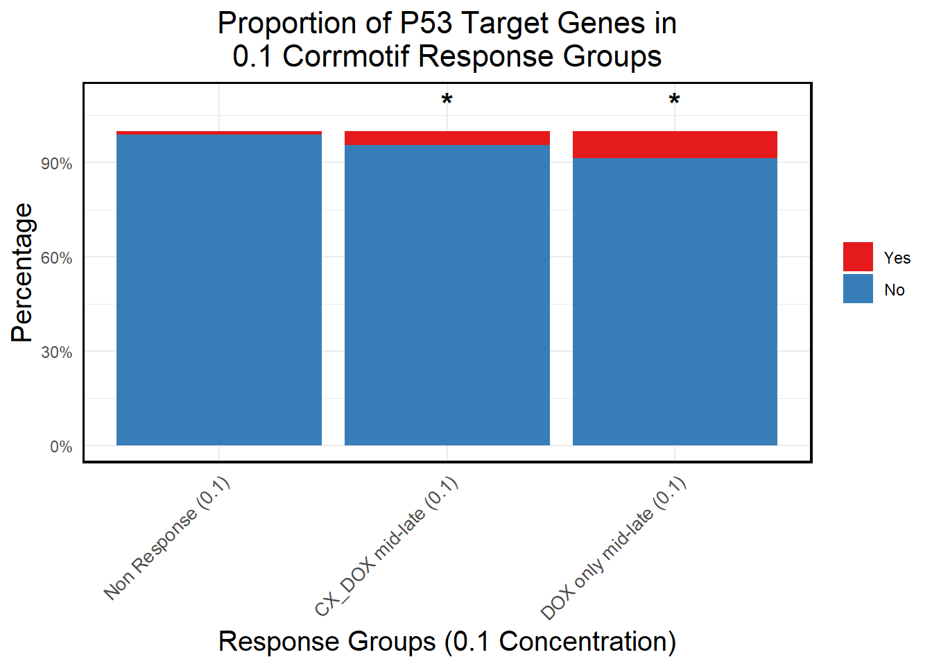
📌 Proportion of P53 target Genes (0.5 micromolar)

# Load necessary libraries
library(dplyr)
library(ggplot2)
library(tidyr)
library(org.Hs.eg.db)

# **🔹 Read P53 Target Gene List**
P53_Target <- read.csv("data/P53_Target.csv", stringsAsFactors = FALSE)

# Convert gene symbols to Entrez IDs
P53_Target <- P53_Target %>%
  mutate(Entrez_ID = mapIds(org.Hs.eg.db,
                            keys = P53_Target$Symbol,
                            column = "ENTREZID",
                            keytype = "SYMBOL",
                            multiVals = "first"))

P53_Target_genes <- na.omit(P53_Target$Entrez_ID)

# **🔹 Load Corrmotif Groups for 0.5 Concentration**
prob_groups_0.5 <- list(
  "Non Response (0.5)" = read.csv("data/prob_1_0.5.csv")$Entrez_ID,
  "DOX-specific response (0.5)" = read.csv("data/prob_2_0.5.csv")$Entrez_ID,
  "DOX only mid-late response (0.5)" = read.csv("data/prob_3_0.5.csv")$Entrez_ID,
  "CX DOX (early) response (0.5)" = read.csv("data/prob_4_0.5.csv")$Entrez_ID,
  "DOX + CX (mid-late) response (0.5)" = read.csv("data/prob_5_0.5.csv")$Entrez_ID
)

# **🔹 Create Dataframe for Corrmotif Groups**
corrmotif_df_0.5 <- bind_rows(
  lapply(prob_groups_0.5, function(ids) {
    data.frame(Entrez_ID = ids)
  }),
  .id = "Response_Group"
)

# **🔹 Match Entrez_IDs with P53 Target Genes**
corrmotif_df_0.5 <- corrmotif_df_0.5 %>%
  mutate(P53_Target = ifelse(Entrez_ID %in% P53_Target_genes, "Yes", "No"))

# **🔹 Count P53 Target Genes in Each Response Group**
proportion_data <- corrmotif_df_0.5 %>%
  group_by(Response_Group, P53_Target) %>%
  summarise(Count = n(), .groups = "drop") %>%
  group_by(Response_Group) %>%
  mutate(Percentage = (Count / sum(Count)) * 100)

# **🔹 Ensure "Yes" is at the Bottom and "No" at the Top**
proportion_data$P53_Target <- factor(proportion_data$P53_Target, levels = c("Yes", "No"))

# **🔹 Set Order of Response Groups for X-axis**
response_order <- c("Non Response (0.5)", "DOX-specific response (0.5)", "DOX only mid-late response (0.5)", 
                    "CX DOX (early) response (0.5)", "DOX + CX (mid-late) response (0.5)")
proportion_data$Response_Group <- factor(proportion_data$Response_Group, levels = response_order)

# **🔹 Perform Chi-Square Tests for Each Response Group vs Non-Response**
non_response_counts <- proportion_data %>%
  filter(Response_Group == "Non Response (0.5)") %>%
  dplyr::select(P53_Target, Count) %>%
  {setNames(.$Count, .$P53_Target)}  # Convert to named vector

# **Comparing Each Group Against "Non Response (0.5)"**
chi_results <- proportion_data %>%
  filter(Response_Group %in% c("DOX-specific response (0.5)", "DOX only mid-late response (0.5)", 
                               "CX DOX (early) response (0.5)", "DOX + CX (mid-late) response (0.5)")) %>%
  group_by(Response_Group) %>%
  summarise(
    p_value = {
      group_counts <- Count[P53_Target %in% c("Yes", "No")]
      if (!"Yes" %in% P53_Target) group_counts <- c(group_counts, 0)
      if (!"No" %in% P53_Target) group_counts <- c(0, group_counts)

      contingency_table <- matrix(c(
        group_counts[1], group_counts[2],  # Response group counts
        non_response_counts["Yes"], non_response_counts["No"]  # Non-response counts
      ), nrow = 2, byrow = TRUE)

      # Perform chi-square test if all values are valid
      if (all(contingency_table >= 0 & is.finite(contingency_table))) {
        chisq.test(contingency_table)$p.value
      } else {
        NA
      }
    },
    .groups = "drop"
  ) %>%
  mutate(Significance = ifelse(!is.na(p_value) & p_value < 0.05, "*", ""))

Warning: There was 1 warning in `summarise()`.
ℹ In argument: `p_value = { ... }`.
ℹ In group 3: `Response_Group = CX DOX (early) response (0.5)`.
Caused by warning in `chisq.test()`:
! Chi-squared approximation may be incorrect

# **🔹 Merge Chi-Square Results into Proportion Data**
proportion_data <- proportion_data %>%
  left_join(chi_results %>% dplyr::select(Response_Group, Significance), by = "Response_Group")

# **🔹 Set Star Position Uniform Across Groups at 105%**
star_positions <- data.frame(
  Response_Group = c("DOX-specific response (0.5)", "DOX only mid-late response (0.5)", 
                     "CX DOX (early) response (0.5)", "DOX + CX (mid-late) response (0.5)"),
  y_pos = 105,  # Fixed at 105% of Y-axis
  Significance = chi_results$Significance
)

# **🔹 Generate Proportion Plot with Chi-Square Stars**
ggplot(proportion_data, aes(x = Response_Group, y = Percentage, fill = P53_Target)) +
  geom_bar(stat = "identity", position = "stack") +  # Stacked bars
  geom_text(
    data = star_positions,
    aes(x = Response_Group, y = y_pos, label = Significance),  # Place stars at fixed 105%
    inherit.aes = FALSE,
    size = 6, color = "black", fontface = "bold", vjust = 0  # Keeps stars aligned
  ) +
  scale_y_continuous(labels = scales::percent_format(scale = 1), limits = c(0, 110)) +  # **Y-axis now limited to 110% for visibility**
  scale_fill_manual(values = c("Yes" = "#e41a1c", "No" = "#377eb8")) +  # Yes (Red), No (Blue)
  labs(
    title = "Proportion of P53 Target Genes in\n0.5 Corrmotif Response Groups",
    x = "Response Groups (0.5 Concentration)",
    y = "Percentage",
    fill = "P53 Target Genes"
  ) +
  theme_minimal() +
  theme(
    plot.title = element_text(size = rel(1.5), hjust = 0.5),
    axis.title = element_text(size = 15, color = "black"),
    axis.text.x = element_text(size = 10, angle = 45, hjust = 1),
    legend.title = element_blank(),
    panel.border = element_rect(color = "black", fill = NA, linewidth = 1.2),
    strip.background = element_blank(),
    strip.text = element_text(size = 12, face = "bold")
  )

Past versions of "prop P53 0.5-1.png"

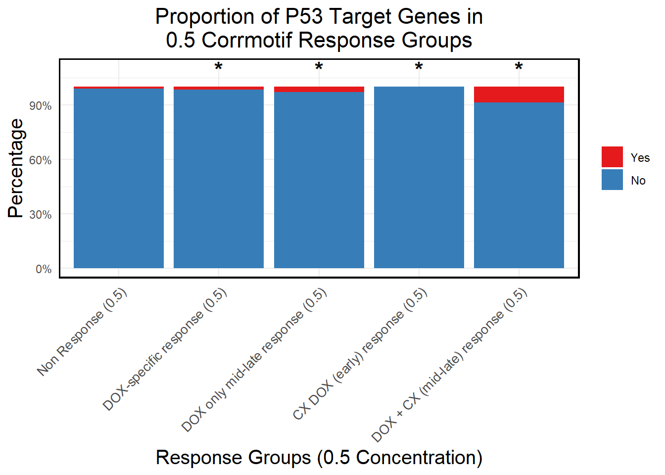
Version	Author	Date
96d0db1	sayanpaul01	2025-03-05

Session information

sessionInfo()

R version 4.3.0 (2023-04-21 ucrt)
Platform: x86_64-w64-mingw32/x64 (64-bit)
Running under: Windows 11 x64 (build 22631)

Matrix products: default


locale:
[1] LC_COLLATE=English_United States.utf8 
[2] LC_CTYPE=English_United States.utf8   
[3] LC_MONETARY=English_United States.utf8
[4] LC_NUMERIC=C                          
[5] LC_TIME=English_United States.utf8    

time zone: America/Chicago
tzcode source: internal

attached base packages:
[1] stats4    stats     graphics  grDevices utils     datasets  methods  
[8] base     

other attached packages:
 [1] org.Hs.eg.db_3.18.0  AnnotationDbi_1.64.1 IRanges_2.36.0      
 [4] S4Vectors_0.40.1     tidyr_1.3.1          ggplot2_3.5.1       
 [7] gprofiler2_0.2.3     BiocParallel_1.36.0  dplyr_1.1.4         
[10] Rfast_2.1.0          RcppParallel_5.1.9   RcppZiggurat_0.1.6  
[13] Rcpp_1.0.12          Cormotif_1.48.0      limma_3.58.1        
[16] affy_1.80.0          Biobase_2.62.0       BiocGenerics_0.48.1 
[19] workflowr_1.7.1     

loaded via a namespace (and not attached):
 [1] tidyselect_1.2.1        viridisLite_0.4.2       farver_2.1.2           
 [4] blob_1.2.4              bitops_1.0-7            Biostrings_2.70.1      
 [7] RCurl_1.98-1.13         fastmap_1.1.1           lazyeval_0.2.2         
[10] promises_1.3.0          digest_0.6.34           lifecycle_1.0.4        
[13] statmod_1.5.0           processx_3.8.5          KEGGREST_1.42.0        
[16] RSQLite_2.3.3           magrittr_2.0.3          compiler_4.3.0         
[19] rlang_1.1.3             sass_0.4.9              tools_4.3.0            
[22] yaml_2.3.10             data.table_1.14.10      knitr_1.49             
[25] labeling_0.4.3          htmlwidgets_1.6.4       bit_4.0.5              
[28] withr_3.0.2             purrr_1.0.2             grid_4.3.0             
[31] preprocessCore_1.64.0   git2r_0.35.0            colorspace_2.1-0       
[34] scales_1.3.0            cli_3.6.1               crayon_1.5.3           
[37] rmarkdown_2.29          generics_0.1.3          rstudioapi_0.17.1      
[40] httr_1.4.7              DBI_1.2.3               cachem_1.0.8           
[43] stringr_1.5.1           zlibbioc_1.48.0         parallel_4.3.0         
[46] XVector_0.42.0          BiocManager_1.30.25     vctrs_0.6.5            
[49] jsonlite_1.8.9          callr_3.7.6             bit64_4.0.5            
[52] plotly_4.10.4           jquerylib_0.1.4         affyio_1.72.0          
[55] glue_1.7.0              codetools_0.2-20        ps_1.8.1               
[58] stringi_1.8.3           gtable_0.3.6            GenomeInfoDb_1.38.8    
[61] later_1.3.2             munsell_0.5.1           tibble_3.2.1           
[64] pillar_1.10.1           htmltools_0.5.8.1       GenomeInfoDbData_1.2.11
[67] R6_2.5.1                rprojroot_2.0.4         evaluate_1.0.3         
[70] png_0.1-8               memoise_2.0.1           httpuv_1.6.15          
[73] bslib_0.8.0             whisker_0.4.1           xfun_0.50              
[76] fs_1.6.3                getPass_0.2-4           pkgconfig_2.0.3