Overlap of GO Terms in DEGs
Last updated: 2025-05-23
Checks: 6 1
Knit directory: CX5461_Project/
This reproducible R Markdown analysis was created with workflowr (version 1.7.1). The Checks tab describes the reproducibility checks that were applied when the results were created. The Past versions tab lists the development history.
The R Markdown file has unstaged changes. To know which version of
the R Markdown file created these results, you’ll want to first commit
it to the Git repo. If you’re still working on the analysis, you can
ignore this warning. When you’re finished, you can run
wflow_publish to commit the R Markdown file and build the
HTML.
Great job! The global environment was empty. Objects defined in the global environment can affect the analysis in your R Markdown file in unknown ways. For reproduciblity it’s best to always run the code in an empty environment.
The command set.seed(20250129) was run prior to running
the code in the R Markdown file. Setting a seed ensures that any results
that rely on randomness, e.g. subsampling or permutations, are
reproducible.
Great job! Recording the operating system, R version, and package versions is critical for reproducibility.
Nice! There were no cached chunks for this analysis, so you can be confident that you successfully produced the results during this run.
Great job! Using relative paths to the files within your workflowr project makes it easier to run your code on other machines.
Great! You are using Git for version control. Tracking code development and connecting the code version to the results is critical for reproducibility.
The results in this page were generated with repository version 3f424e4. See the Past versions tab to see a history of the changes made to the R Markdown and HTML files.
Note that you need to be careful to ensure that all relevant files for
the analysis have been committed to Git prior to generating the results
(you can use wflow_publish or
wflow_git_commit). workflowr only checks the R Markdown
file, but you know if there are other scripts or data files that it
depends on. Below is the status of the Git repository when the results
were generated:
Ignored files:
    Ignored:    .RData
    Ignored:    .Rhistory
    Ignored:    .Rproj.user/
    Ignored:    0.1 box.svg
    Ignored:    Rplot04.svg
    Ignored:    analysis/Corrmotif_Conc.html

Untracked files:
    Untracked:  0.1 density.svg
    Untracked:  0.1.emf
    Untracked:  0.1.svg
    Untracked:  0.5 box.svg
    Untracked:  0.5 density.svg
    Untracked:  0.5.svg
    Untracked:  Additional/
    Untracked:  CX_5461_Pattern_Genes_24hr.csv
    Untracked:  CX_5461_Pattern_Genes_3hr.csv
    Untracked:  Cell viability box plot.svg
    Untracked:  DRC1.svg
    Untracked:  Figure 1.jpeg
    Untracked:  Figure 1.pdf
    Untracked:  Figure_CM_Purity.pdf
    Untracked:  Rplot.svg
    Untracked:  Rplot01.svg
    Untracked:  Rplot02.svg
    Untracked:  Rplot03.svg
    Untracked:  Rplot05.svg
    Untracked:  Rplot06.svg
    Untracked:  Rplot07.svg
    Untracked:  Rplot08.jpeg
    Untracked:  Rplot08.svg
    Untracked:  Rplot09.svg
    Untracked:  Rplot10.svg
    Untracked:  Rplot11.svg
    Untracked:  Rplot12.svg
    Untracked:  Rplot13.svg
    Untracked:  Rplot14.svg
    Untracked:  TOP2B.bed
    Untracked:  TS HPA (Violin).svg
    Untracked:  TS HPA.svg
    Untracked:  TS_HA.svg
    Untracked:  TS_HV.svg
    Untracked:  Violin HA.svg
    Untracked:  Violin HV (CX vs DOX).svg
    Untracked:  Violin HV.svg
    Untracked:  data/AF.csv
    Untracked:  data/AF_Mapped.csv
    Untracked:  data/AF_genes.csv
    Untracked:  data/Annotated_DOX_Gene_Table.csv
    Untracked:  data/BP/
    Untracked:  data/CAD_genes.csv
    Untracked:  data/Cardiotox.csv
    Untracked:  data/Cardiotox_mapped.csv
    Untracked:  data/DOX_Vald.csv
    Untracked:  data/DOX_Vald_Mapped.csv
    Untracked:  data/DOX_alt.csv
    Untracked:  data/Entrez_Cardiotox.csv
    Untracked:  data/Entrez_Cardiotox_Mapped.csv
    Untracked:  data/GWAS.xlsx
    Untracked:  data/GWAS_SNPs.bed
    Untracked:  data/HF.csv
    Untracked:  data/HF_Mapped.csv
    Untracked:  data/HF_genes.csv
    Untracked:  data/Hypertension_genes.csv
    Untracked:  data/MI_genes.csv
    Untracked:  data/P53_Target_mapped.csv
    Untracked:  data/Sample_annotated.csv
    Untracked:  data/Samples.csv
    Untracked:  data/Samples.xlsx
    Untracked:  data/TOP2A.bed
    Untracked:  data/TOP2A_target.csv
    Untracked:  data/TOP2A_target_lit.csv
    Untracked:  data/TOP2A_target_lit_mapped.csv
    Untracked:  data/TOP2A_target_mapped.csv
    Untracked:  data/TOP2B.bed
    Untracked:  data/TOP2B_target.csv
    Untracked:  data/TOP2B_target_heatmap.csv
    Untracked:  data/TOP2B_target_heatmap_mapped.csv
    Untracked:  data/TOP2B_target_mapped.csv
    Untracked:  data/TS.csv
    Untracked:  data/TS_HPA.csv
    Untracked:  data/TS_HPA_mapped.csv
    Untracked:  data/Toptable_CX_0.1_24.csv
    Untracked:  data/Toptable_CX_0.1_3.csv
    Untracked:  data/Toptable_CX_0.1_48.csv
    Untracked:  data/Toptable_CX_0.5_24.csv
    Untracked:  data/Toptable_CX_0.5_3.csv
    Untracked:  data/Toptable_CX_0.5_48.csv
    Untracked:  data/Toptable_DOX_0.1_24.csv
    Untracked:  data/Toptable_DOX_0.1_3.csv
    Untracked:  data/Toptable_DOX_0.1_48.csv
    Untracked:  data/Toptable_DOX_0.5_24.csv
    Untracked:  data/Toptable_DOX_0.5_3.csv
    Untracked:  data/Toptable_DOX_0.5_48.csv
    Untracked:  data/count.tsv
    Untracked:  data/ts_data_mapped
    Untracked:  results/
    Untracked:  run_bedtools.bat

Unstaged changes:
    Deleted:    analysis/Actox.Rmd
    Modified:   analysis/Overlap_GO_DEG.Rmd
    Modified:   data/count.csv
Note that any generated files, e.g. HTML, png, CSS, etc., are not included in this status report because it is ok for generated content to have uncommitted changes.
These are the previous versions of the repository in which changes were
made to the R Markdown (analysis/Overlap_GO_DEG.Rmd) and
HTML (docs/Overlap_GO_DEG.html) files. If you’ve configured
a remote Git repository (see ?wflow_git_remote), click on
the hyperlinks in the table below to view the files as they were in that
past version.
| File | Version | Author | Date | Message |
|---|---|---|---|---|
| html | bb4b782 | sayanpaul01 | 2025-02-20 | Build site. |
| html | 2e99243 | sayanpaul01 | 2025-02-20 | Build site. |
| Rmd | 7f9dc02 | sayanpaul01 | 2025-02-20 | Added Overlap of GO Terms in DEGs and updated index |
📌 Load Required Libraries
library(ggVennDiagram)
library(ggplot2)
library(dplyr)
📌 Read and Process GO Terms
# Load GO term data for different conditions
# Load GO term data for different conditions
CX_0.1_24_GO <- read.csv("data/CX_0.1_24 (Combined).csv")
CX_0.1_48_GO <- read.csv("data/CX_0.1_48 (Combined).csv")
CX_0.5_3_GO  <- read.csv("data/CX_0.5_3 (Combined).csv")
CX_0.5_24_GO <- read.csv("data/CX_0.5_24 (Combined).csv")
CX_0.5_48_GO <- read.csv("data/CX_0.5_48 (Combined).csv")

DOX_0.1_3_GO  <- read.csv("data/DOX_0.1_3 (Combined).csv")
DOX_0.1_24_GO <- read.csv("data/DOX_0.1_24 (Combined).csv")
DOX_0.1_48_GO <- read.csv("data/DOX_0.1_48 (Combined).csv")
DOX_0.5_3_GO  <- read.csv("data/DOX_0.5_3 (Combined).csv")
DOX_0.5_24_GO <- read.csv("data/DOX_0.5_24 (Combined).csv")
DOX_0.5_48_GO <- read.csv("data/DOX_0.5_48 (Combined).csv")

# Extract GO term IDs for each condition
DEG2_GO <- CX_0.1_24_GO$ID
DEG3_GO <- CX_0.1_48_GO$ID
DEG4_GO <- CX_0.5_3_GO$ID
DEG5_GO <- CX_0.5_24_GO$ID
DEG6_GO <- CX_0.5_48_GO$ID
DEG7_GO <- DOX_0.1_3_GO$ID
DEG8_GO <- DOX_0.1_24_GO$ID
DEG9_GO <- DOX_0.1_48_GO$ID
DEG10_GO <- DOX_0.5_3_GO$ID
DEG11_GO <- DOX_0.5_24_GO$ID
DEG12_GO <- DOX_0.5_48_GO$term_id
📌 Overlap of GO Terms across the drugs
📌 Overlap of GO Terms in CX-5461 vs VEH
CX_Datasets <- list(
  "CX_0.1_24" = DEG2_GO,
  "CX_0.1_48" = DEG3_GO,
  "CX_0.5_3" = DEG4_GO,
  "CX_0.5_24" = DEG5_GO,
  "CX_0.5_48" = DEG6_GO
)

ggVennDiagram(CX_Datasets, label = "count") +
  theme(
    plot.title = element_text(size = 16, face = "bold"),
    legend.title = element_text(size = 12, face = "bold"),
    legend.text = element_text(size = 10)
  ) +
  labs(title = "CX-5461 GO Term Overlap")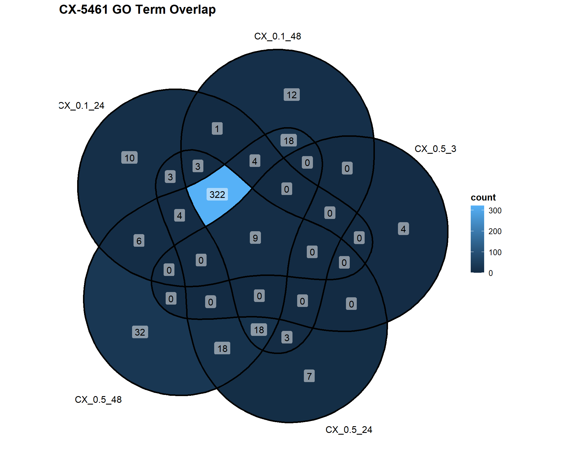
| Version | Author | Date |
|---|---|---|
| 2e99243 | sayanpaul01 | 2025-02-20 |
📌 Overlap of GO Terms in DOX vs VEH
DOX_Datasets <- list(
  "DOX_0.1_3" = DEG7_GO,
  "DOX_0.1_24" = DEG8_GO,
  "DOX_0.1_48" = DEG9_GO,
  "DOX_0.5_3" = DEG10_GO,
  "DOX_0.5_24" = DEG11_GO,
  "DOX_0.5_48" = DEG12_GO
)

ggVennDiagram(DOX_Datasets, label = "count") +
  theme(
    plot.title = element_text(size = 16, face = "bold"),
    legend.title = element_text(size = 12, face = "bold"),
    legend.text = element_text(size = 10)
  ) +
  labs(title = "DOX GO Term Overlap")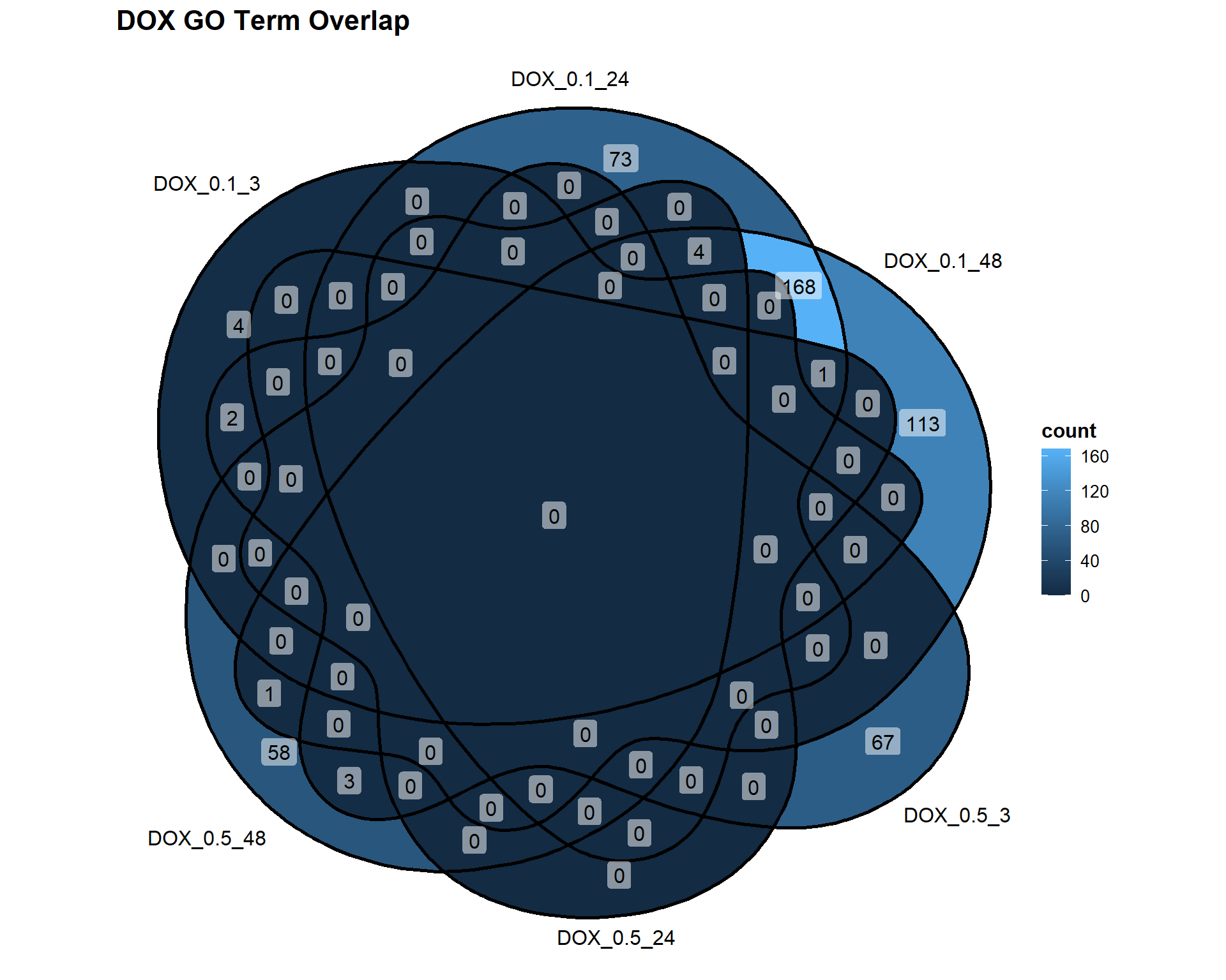
| Version | Author | Date |
|---|---|---|
| 2e99243 | sayanpaul01 | 2025-02-20 |
📌 Overlap of GO Terms across concentrations
📌 0.1 µM Concentration
Concentration_0_1 <- list(
  "CX_0.1_24" = DEG2_GO,
  "CX_0.1_48" = DEG3_GO,
  "DOX_0.1_3" = DEG7_GO,
  "DOX_0.1_24" = DEG8_GO,
  "DOX_0.1_48" = DEG9_GO
)

ggVennDiagram(Concentration_0_1, label = "count") +
  theme(
    plot.title = element_text(size = 16, face = "bold"),
    legend.title = element_text(size = 12, face = "bold"),
    legend.text = element_text(size = 10)
  ) +
  labs(title = "0.1 µM GO Term Overlap")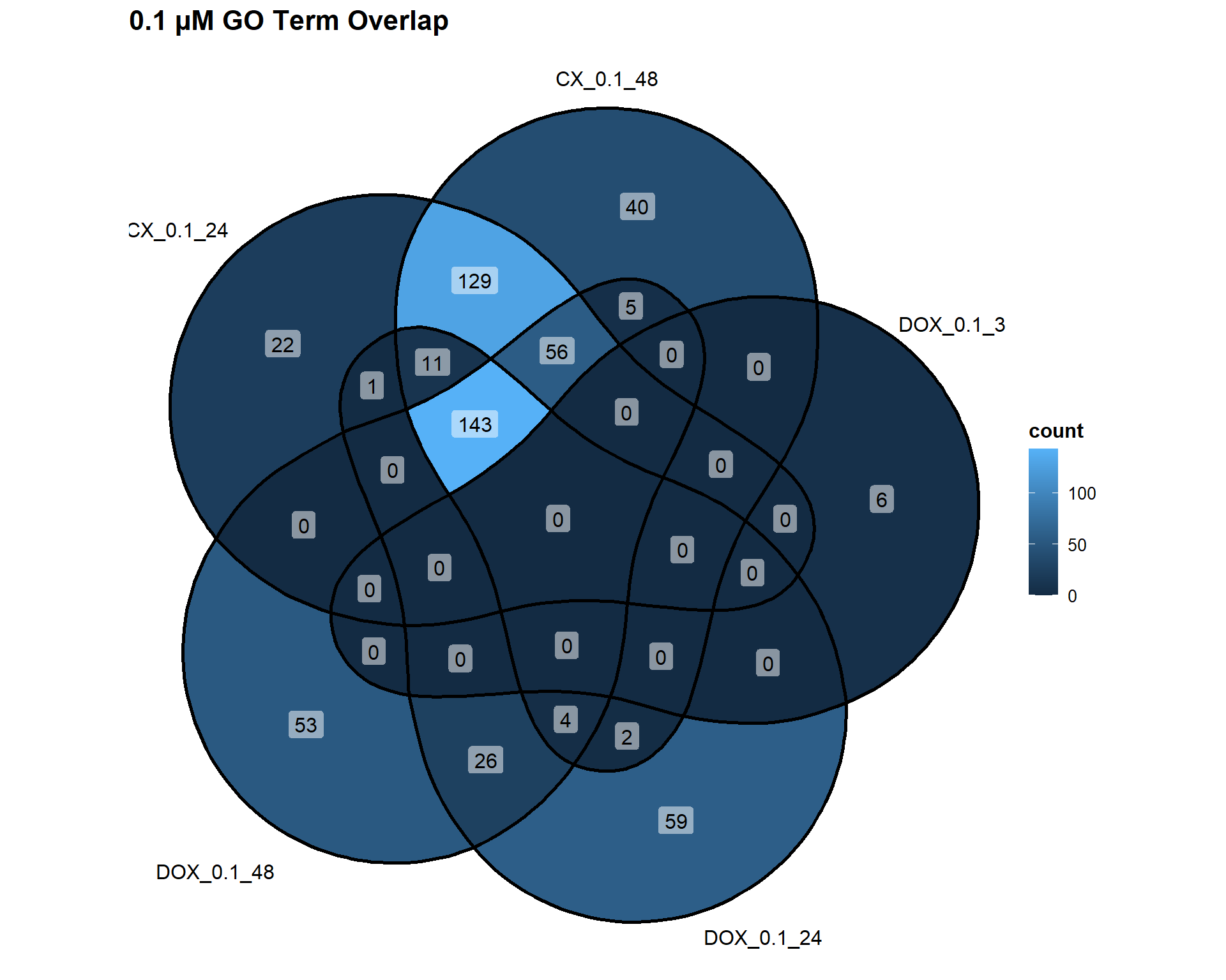
| Version | Author | Date |
|---|---|---|
| 2e99243 | sayanpaul01 | 2025-02-20 |
📌 0.5 µM Concentration
Concentration_0_5 <- list(
  "CX_0.5_3" = DEG4_GO,
  "CX_0.5_24" = DEG5_GO,
  "CX_0.5_48" = DEG6_GO,
  "DOX_0.5_3" = DEG10_GO,
  "DOX_0.5_24" = DEG11_GO,
  "DOX_0.5_48" = DEG12_GO
)

ggVennDiagram(Concentration_0_5, label = "count") +
  theme(
    plot.title = element_text(size = 16, face = "bold"),
    legend.title = element_text(size = 12, face = "bold"),
    legend.text = element_text(size = 10)
  ) +
  labs(title = "0.5 µM GO Term Overlap")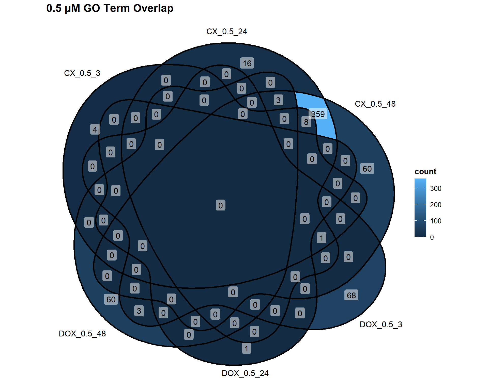
| Version | Author | Date |
|---|---|---|
| 2e99243 | sayanpaul01 | 2025-02-20 |
📌 Overlap of GO Terms Across Timepoints
📌3 Hours
Timepoint_3hrs <- list(
  "CX_0.5_3" = DEG4_GO,
  "DOX_0.1_3" = DEG7_GO,
  "DOX_0.5_3" = DEG10_GO
)

ggVennDiagram(Timepoint_3hrs, label = "count") +
  theme(
    plot.title = element_text(size = 16, face = "bold"),
    legend.title = element_text(size = 12, face = "bold"),
    legend.text = element_text(size = 10)
  ) +
  labs(title = "3 Hours GO Term Overlap")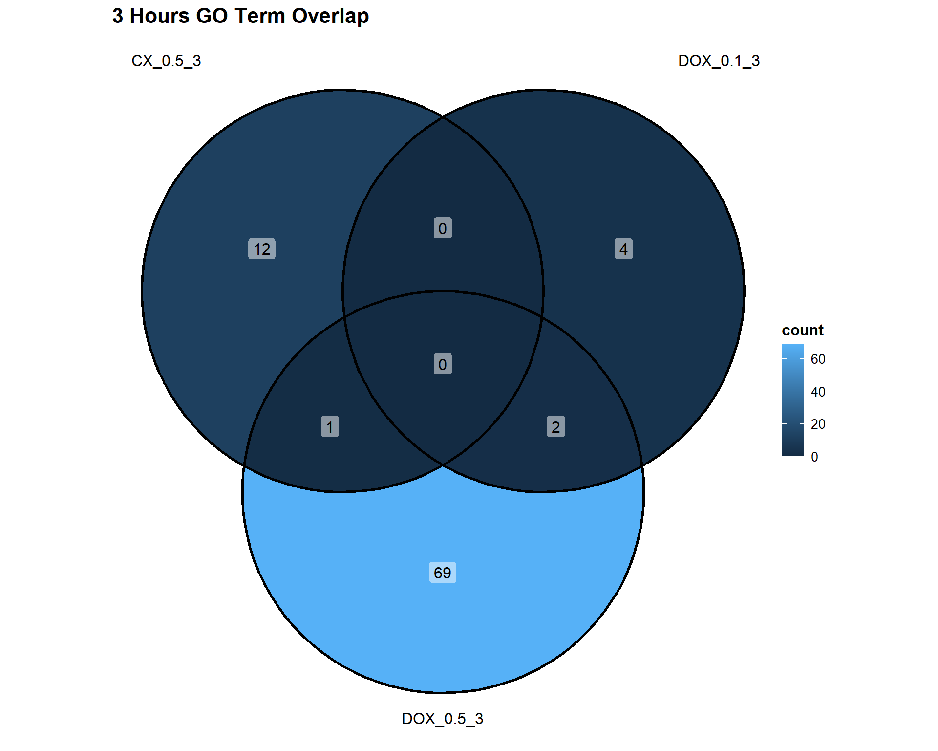
| Version | Author | Date |
|---|---|---|
| 2e99243 | sayanpaul01 | 2025-02-20 |
📌24 Hours
Timepoint_24hrs <- list(
  "CX_0.1_24" = DEG2_GO,
  "CX_0.5_24" = DEG5_GO,
  "DOX_0.1_24" = DEG8_GO,
  "DOX_0.5_24" = DEG11_GO
)

ggVennDiagram(Timepoint_24hrs, label = "count") +
  theme(
    plot.title = element_text(size = 16, face = "bold"),
    legend.title = element_text(size = 12, face = "bold"),
    legend.text = element_text(size = 10)
  ) +
  labs(title = "24 Hours GO Term Overlap")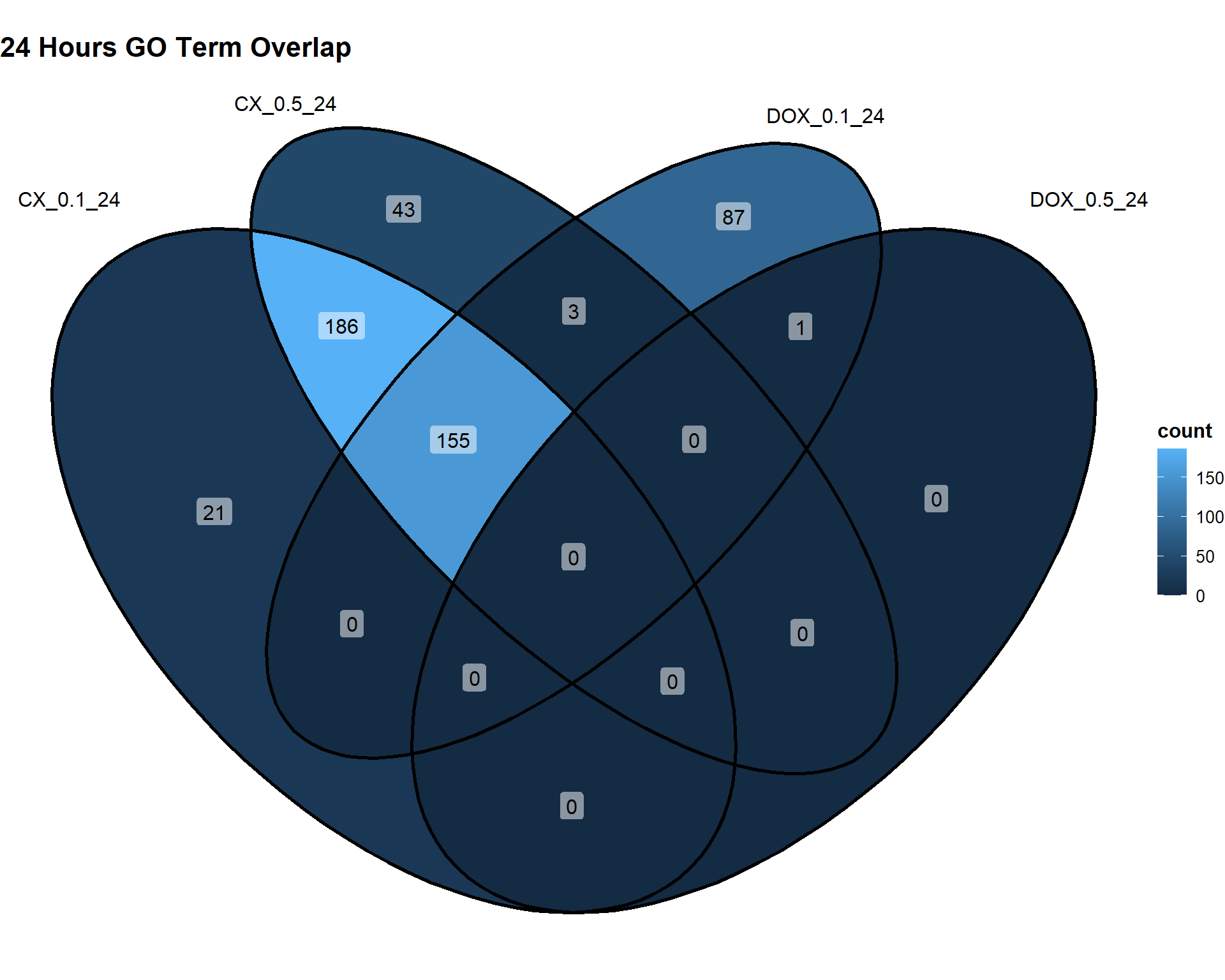
| Version | Author | Date |
|---|---|---|
| 2e99243 | sayanpaul01 | 2025-02-20 |
📌48 Hours
Timepoint_48hrs <- list(
  "CX_0.1_48" = DEG3_GO,
  "CX_0.5_48" = DEG6_GO,
  "DOX_0.1_48" = DEG9_GO,
  "DOX_0.5_48" = DEG12_GO
)

ggVennDiagram(Timepoint_48hrs, label = "count") +
  theme(
    plot.title = element_text(size = 16, face = "bold"),
    legend.title = element_text(size = 12, face = "bold"),
    legend.text = element_text(size = 10)
  ) +
  labs(title = "48 Hours GO Term Overlap")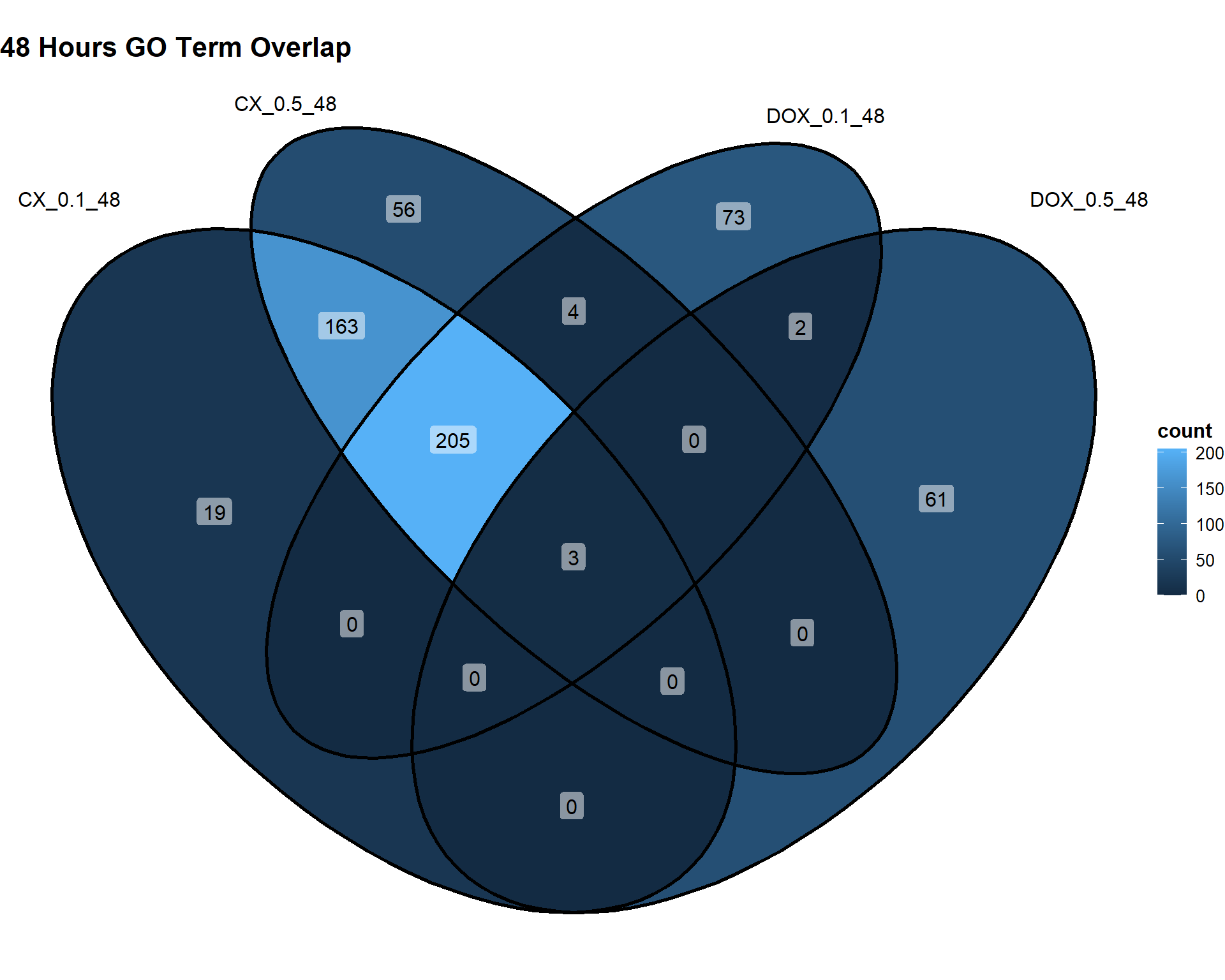
| Version | Author | Date |
|---|---|---|
| 2e99243 | sayanpaul01 | 2025-02-20 |
📌Overlapping of GO terms across all samples Upset plot
# 📦 Load Required Libraries
library(UpSetR)
library(dplyr)
library(tidyr)

# ✅ Load all GO term datasets
CX_0.1_24_GO <- read.csv("data/BP/CX_0.1_24 (Combined).csv")
CX_0.1_48_GO <- read.csv("data/BP/CX_0.1_48 (Combined).csv")
CX_0.5_3_GO  <- read.csv("data/BP/CX_0.5_3 (Combined).csv")
CX_0.5_24_GO <- read.csv("data/BP/CX_0.5_24 (Combined).csv")
CX_0.5_48_GO <- read.csv("data/BP/CX_0.5_48 (Combined).csv")
DOX_0.1_3_GO <- read.csv("data/BP/DOX_0.1_3 (Combined).csv")
DOX_0.1_24_GO <- read.csv("data/BP/DOX_0.1_24 (Combined).csv")
DOX_0.1_48_GO <- read.csv("data/BP/DOX_0.1_48 (Combined).csv")
DOX_0.5_3_GO <- read.csv("data/BP/DOX_0.5_3 (Combined).csv")

# ✅ Prepare list of GO IDs
gene_sets <- list(
  `CX_0.1_24` = as.character(CX_0.1_24_GO$ID),
  `CX_0.1_48` = as.character(CX_0.1_48_GO$ID),
  `CX_0.5_3`  = as.character(CX_0.5_3_GO$ID),
  `CX_0.5_24` = as.character(CX_0.5_24_GO$ID),
  `CX_0.5_48` = as.character(CX_0.5_48_GO$ID),
  `DOX_0.1_3` = as.character(DOX_0.1_3_GO$ID),
  `DOX_0.1_24` = as.character(DOX_0.1_24_GO$ID),
  `DOX_0.1_48` = as.character(DOX_0.1_48_GO$ID),
  `DOX_0.5_3` = as.character(DOX_0.5_3_GO$ID)
)

# 🧮 Build binary matrix
all_ids <- unique(unlist(gene_sets))
binary_matrix <- data.frame(GO_ID = all_ids)

for (name in names(gene_sets)) {
  binary_matrix[[name]] <- as.integer(binary_matrix$GO_ID %in% gene_sets[[name]])
}

# ✅ Remove GO_ID for upset input
upset_input <- binary_matrix[, -1]
colnames(upset_input) <- names(gene_sets)  # ensure consistent names

# ✅ Plot
par(mar = c(10, 4, 2, 2))  # bottom, left, top, right
upset(upset_input,
      sets = colnames(upset_input),
      order.by = "freq",
      sets.bar.color = "#56B4E9",
      mainbar.y.label = "Number of Shared BP",
      sets.x.label = "BP per Condition",
      text.scale = 1.2,
      nintersects = 30)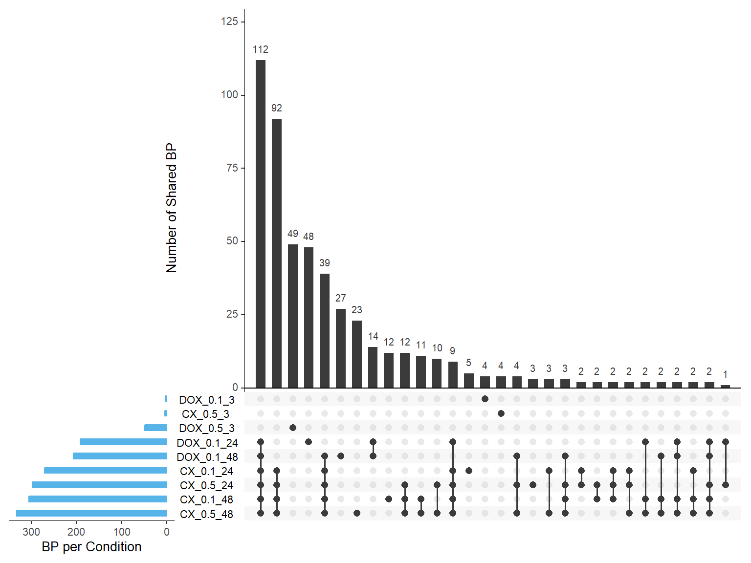
📌Identifying Unique GO terms
# 📦 Load Required Libraries
library(dplyr)
library(readr)

# ✅ Step 1: Load GO Enrichment Files
CX_0.1_24_GO <- read_csv("data/BP/CX_0.1_24 (Combined).csv")
CX_0.1_48_GO <- read_csv("data/BP/CX_0.1_48 (Combined).csv")
CX_0.5_3_GO  <- read_csv("data/BP/CX_0.5_3 (Combined).csv")
CX_0.5_24_GO <- read_csv("data/BP/CX_0.5_24 (Combined).csv")
CX_0.5_48_GO <- read_csv("data/BP/CX_0.5_48 (Combined).csv")
DOX_0.1_3_GO <- read_csv("data/BP/DOX_0.1_3 (Combined).csv")
DOX_0.1_24_GO <- read_csv("data/BP/DOX_0.1_24 (Combined).csv")
DOX_0.1_48_GO <- read_csv("data/BP/DOX_0.1_48 (Combined).csv")
DOX_0.5_3_GO <- read_csv("data/BP/DOX_0.5_3 (Combined).csv")

# ✅ Step 2: Create Named List of Data Frames
go_files <- list(
  `CX_0.1_24` = CX_0.1_24_GO,
  `CX_0.1_48` = CX_0.1_48_GO,
  `CX_0.5_3`  = CX_0.5_3_GO,
  `CX_0.5_24` = CX_0.5_24_GO,
  `CX_0.5_48` = CX_0.5_48_GO,
  `DOX_0.1_3` = DOX_0.1_3_GO,
  `DOX_0.1_24` = DOX_0.1_24_GO,
  `DOX_0.1_48` = DOX_0.1_48_GO,
  `DOX_0.5_3` = DOX_0.5_3_GO
)

# ✅ Step 3: Find Unique GO IDs for Each Condition
unique_go_terms <- list()

for (set_name in names(go_files)) {
  current_ids <- go_files[[set_name]]$ID
  other_ids <- unlist(go_files[names(go_files) != set_name], use.names = FALSE)
  unique_ids <- setdiff(current_ids, other_ids)

  if (length(unique_ids) > 0) {
    unique_go_terms[[set_name]] <- unique_ids
  }
}

# ✅ Step 4: Map Unique GO IDs to Descriptions and p.adjust
mapped_unique_go_terms <- list()

for (set_name in names(unique_go_terms)) {
  source_df <- go_files[[set_name]]
  unique_ids <- unique_go_terms[[set_name]]

  mapped_df <- source_df %>%
    filter(ID %in% unique_ids) %>%
    dplyr::select(GO_ID = ID, Function = Description, p.adjust)

  mapped_unique_go_terms[[set_name]] <- mapped_df
}

# 🎯 Final Output: List of data.frames with GO_ID, Description, and p.adjust
mapped_unique_go_terms
$CX_0.1_24
# A tibble: 5 × 3
GO_ID Function p.adjust
<chr> <chr> <dbl>
1 GO:0032147 activation of protein kinase activity 0.0163
2 GO:0061351 neural precursor cell proliferation 0.0173
3 GO:0030865 cortical cytoskeleton organization 0.0295
4 GO:0021987 cerebral cortex development 0.0296
5 GO:0007283 spermatogenesis 0.0438
$CX_0.1_48
# A tibble: 12 × 3
GO_ID Function p.adjust
<chr> <chr> <dbl>
1 GO:1902115 regulation of organelle assembly 0.0237
2 GO:0009994 oocyte differentiation 0.0301
3 GO:0007281 germ cell development 0.0345
4 GO:0048469 cell maturation 0.0369
5 GO:0070979 protein K11-linked ubiquitination 0.0390
6 GO:0007141 male meiosis I 0.0393
7 GO:0046653 tetrahydrofolate metabolic process 0.0393
8 GO:0042558 pteridine-containing compound metabolic process 0.0434
9 GO:0048477 oogenesis 0.0437
10 GO:0006266 DNA ligation 0.0462
11 GO:0009163 nucleoside biosynthetic process 0.0462
12 GO:0034404 nucleobase-containing small molecule biosynthetic process 0.0462
$CX_0.5_3
# A tibble: 4 × 3
GO_ID Function p.adjust
<chr> <chr> <dbl>
1 GO:0060218 hematopoietic stem cell differentiation 0.0123
2 GO:0002244 hematopoietic progenitor cell differentiation 0.0145
3 GO:0048863 stem cell differentiation 0.0200
4 GO:0007517 muscle organ development 0.0228
$CX_0.5_24
# A tibble: 3 × 3
GO_ID Function p.adjust
<chr> <chr> <dbl>
1 GO:0008630 intrinsic apoptotic signaling pathway in response to DNA … 0.0196
2 GO:0071539 protein localization to centrosome 0.0330
3 GO:1905508 protein localization to microtubule organizing center 0.0363
$CX_0.5_48
# A tibble: 23 × 3
GO_ID Function p.adjust
<chr> <chr> <dbl>
1 GO:0031507 heterochromatin formation 0.000678
2 GO:0070828 heterochromatin organization 0.00134
3 GO:0032200 telomere organization 0.00509
4 GO:0006305 DNA alkylation 0.00675
5 GO:0006306 DNA methylation 0.00675
6 GO:0009129 pyrimidine nucleoside monophosphate metabolic process 0.00985
7 GO:0051446 positive regulation of meiotic cell cycle 0.00985
8 GO:0031100 animal organ regeneration 0.0137
9 GO:0009219 pyrimidine deoxyribonucleotide metabolic process 0.0148
10 GO:0006544 glycine metabolic process 0.0189
# ℹ 13 more rows
$DOX_0.1_3
# A tibble: 4 × 3
GO_ID Function p.adjust
<chr> <chr> <dbl>
1 GO:1900034 regulation of cellular response to heat 0.0105
2 GO:0034605 cellular response to heat 0.0167
3 GO:0009408 response to heat 0.0172
4 GO:0009266 response to temperature stimulus 0.0203
$DOX_0.1_24
# A tibble: 48 × 3
GO_ID Function p.adjust
<chr> <chr> <dbl>
1 GO:0070372 regulation of ERK1 and ERK2 cascade 0.000752
2 GO:0001759 organ induction 0.00146
3 GO:0070371 ERK1 and ERK2 cascade 0.00185
4 GO:0032609 type II interferon production 0.00247
5 GO:0032649 regulation of type II interferon production 0.00247
6 GO:0008585 female gonad development 0.00284
7 GO:0061458 reproductive system development 0.00335
8 GO:0010712 regulation of collagen metabolic process 0.00427
9 GO:0048608 reproductive structure development 0.00440
10 GO:0046545 development of primary female sexual characteristics 0.00536
# ℹ 38 more rows
$DOX_0.1_48
# A tibble: 27 × 3
GO_ID Function p.adjust
<chr> <chr> <dbl>
1 GO:1901136 carbohydrate derivative catabolic process 0.000105
2 GO:0006516 glycoprotein catabolic process 0.000480
3 GO:0008045 motor neuron axon guidance 0.00661
4 GO:0030903 notochord development 0.00992
5 GO:0086010 membrane depolarization during action potential 0.0162
6 GO:0034644 cellular response to UV 0.0162
7 GO:0001508 action potential 0.0164
8 GO:0043062 extracellular structure organization 0.0168
9 GO:0097205 renal filtration 0.0211
10 GO:0051899 membrane depolarization 0.0220
# ℹ 17 more rows
$DOX_0.5_3
# A tibble: 49 × 3
GO_ID Function p.adjust
<chr> <chr> <dbl>
1 GO:0060411 cardiac septum morphogenesis 0.0186
2 GO:0003007 heart morphogenesis 0.0186
3 GO:0060840 artery development 0.0186
4 GO:0035270 endocrine system development 0.0186
5 GO:0030098 lymphocyte differentiation 0.0186
6 GO:0003279 cardiac septum development 0.0186
7 GO:0045165 cell fate commitment 0.0207
8 GO:0090092 regulation of transmembrane receptor protein serine/thre… 0.0207
9 GO:0003281 ventricular septum development 0.0207
10 GO:0048844 artery morphogenesis 0.0207
# ℹ 39 more rows📌TOP Unique GO terms
# 📦 Load Required Libraries
library(dplyr)
library(ggplot2)
library(ggpubr)
library(stringr)

# 🧾 mapped_unique_go_terms must already be defined from your previous step:
# List of data frames with GO_ID, Function, p.adjust

# 🔁 Step 1: Prepare top 10 unique terms per sample
plot_data <- list()

for (set_name in names(mapped_unique_go_terms)) {
  unique_df <- mapped_unique_go_terms[[set_name]]

  if (nrow(unique_df) > 0) {
    unique_df$Sample <- set_name
    unique_df$NegLog10Padj <- -log10(unique_df$p.adjust)

    top10 <- unique_df %>%
      dplyr::slice_min(order_by = p.adjust, n = 10, with_ties = FALSE) %>%
      dplyr::select(Sample, Function, NegLog10Padj)

    plot_data[[set_name]] <- top10
  }
}

# 🔗 Step 2: Combine all and format
plot_df <- bind_rows(plot_data)
plot_df$Function <- str_trunc(plot_df$Function, 60)

# 🎨 Step 3: Plot
ggplot(plot_df, aes(x = NegLog10Padj, y = reorder(Function, NegLog10Padj))) +
  geom_bar(stat = "identity", fill = "#3182bd") +
  facet_wrap(~ Sample, scales = "free_y", ncol = 2, strip.position = "top") +
  labs(x = "-log10(p.adjust)", y = "GO Term", title = "Top Unique GO BP Terms per Sample") +
  theme_pubr(base_size = 14) +
  theme(strip.background = element_rect(colour = "black", fill = "grey90", size = 1),
        strip.text = element_text(face = "bold"),
        axis.text.y = element_text(size = 10),
        panel.border = element_rect(color = "black", fill = NA, size = 1))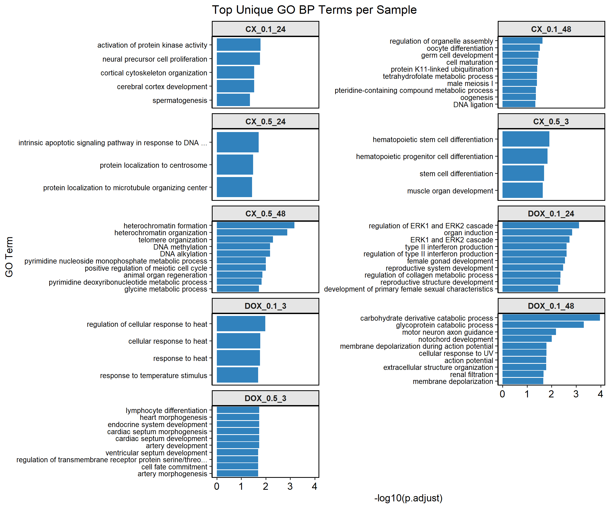
sessionInfo()R version 4.3.0 (2023-04-21 ucrt)
Platform: x86_64-w64-mingw32/x64 (64-bit)
Running under: Windows 11 x64 (build 26100)
Matrix products: default
locale:
[1] LC_COLLATE=English_United States.utf8
[2] LC_CTYPE=English_United States.utf8
[3] LC_MONETARY=English_United States.utf8
[4] LC_NUMERIC=C
[5] LC_TIME=English_United States.utf8
time zone: America/Chicago
tzcode source: internal
attached base packages:
[1] stats graphics grDevices utils datasets methods base
other attached packages:
[1] stringr_1.5.1 ggpubr_0.6.0 readr_2.1.5
[4] tidyr_1.3.1 UpSetR_1.4.0 dplyr_1.1.4
[7] ggplot2_3.5.2 ggVennDiagram_1.5.2
loaded via a namespace (and not attached):
[1] utf8_1.2.4 sass_0.4.10 generics_0.1.3 rstatix_0.7.2
[5] stringi_1.8.3 hms_1.1.3 digest_0.6.34 magrittr_2.0.3
[9] evaluate_1.0.3 grid_4.3.0 fastmap_1.2.0 rprojroot_2.0.4
[13] workflowr_1.7.1 plyr_1.8.9 jsonlite_2.0.0 whisker_0.4.1
[17] backports_1.5.0 Formula_1.2-5 gridExtra_2.3 promises_1.3.2
[21] purrr_1.0.4 scales_1.3.0 jquerylib_0.1.4 abind_1.4-8
[25] cli_3.6.1 crayon_1.5.3 rlang_1.1.3 bit64_4.6.0-1
[29] munsell_0.5.1 withr_3.0.2 cachem_1.1.0 yaml_2.3.10
[33] parallel_4.3.0 tools_4.3.0 tzdb_0.5.0 ggsignif_0.6.4
[37] colorspace_2.1-0 httpuv_1.6.15 broom_1.0.8 vctrs_0.6.5
[41] R6_2.6.1 lifecycle_1.0.4 git2r_0.36.2 car_3.1-3
[45] bit_4.6.0 fs_1.6.3 vroom_1.6.5 pkgconfig_2.0.3
[49] pillar_1.10.2 bslib_0.9.0 later_1.3.2 gtable_0.3.6
[53] glue_1.7.0 Rcpp_1.0.12 xfun_0.52 tibble_3.2.1
[57] tidyselect_1.2.1 rstudioapi_0.17.1 knitr_1.50 farver_2.1.2
[61] htmltools_0.5.8.1 carData_3.0-5 rmarkdown_2.29 labeling_0.4.3
[65] compiler_4.3.0