Chapter 2 - Workflow basics

Last updated: 2020-10-18

Checks: 7 0

Knit directory: r4ds_book/

This reproducible R Markdown analysis was created with workflowr (version 1.6.2). The Checks tab describes the reproducibility checks that were applied when the results were created. The Past versions tab lists the development history.

R Markdown file: up-to-date

Great! Since the R Markdown file has been committed to the Git repository, you know the exact version of the code that produced these results.

Environment: empty

Great job! The global environment was empty. Objects defined in the global environment can affect the analysis in your R Markdown file in unknown ways. For reproduciblity it’s best to always run the code in an empty environment.

Seed: set.seed(20200814)

The command set.seed(20200814) was run prior to running the code in the R Markdown file. Setting a seed ensures that any results that rely on randomness, e.g. subsampling or permutations, are reproducible.

Session information: recorded

Great job! Recording the operating system, R version, and package versions is critical for reproducibility.

Cache: none

Nice! There were no cached chunks for this analysis, so you can be confident that you successfully produced the results during this run.

File paths: relative

Great job! Using relative paths to the files within your workflowr project makes it easier to run your code on other machines.

Repository version: 03b054a

Great! You are using Git for version control. Tracking code development and connecting the code version to the results is critical for reproducibility.

The results in this page were generated with repository version 03b054a. See the Past versions tab to see a history of the changes made to the R Markdown and HTML files.

Note that you need to be careful to ensure that all relevant files for the analysis have been committed to Git prior to generating the results (you can use wflow_publish or wflow_git_commit). workflowr only checks the R Markdown file, but you know if there are other scripts or data files that it depends on. Below is the status of the Git repository when the results were generated:


Ignored files:
    Ignored:    .Rproj.user/

Untracked files:
    Untracked:  VideoDecodeStats/
    Untracked:  analysis/images/
    Untracked:  code_snipp.txt

Note that any generated files, e.g. HTML, png, CSS, etc., are not included in this status report because it is ok for generated content to have uncommitted changes.

These are the previous versions of the repository in which changes were made to the R Markdown (analysis/ch2_workflow.Rmd) and HTML (docs/ch2_workflow.html) files. If you’ve configured a remote Git repository (see ?wflow_git_remote), click on the hyperlinks in the table below to view the files as they were in that past version.

File	Version	Author	Date	Message
html	ce8c214	sciencificity	2020-10-16	Build site.
html	1fa6c06	sciencificity	2020-10-16	Build site.
html	9ae5861	sciencificity	2020-10-13	Build site.
html	76c2bc4	sciencificity	2020-10-10	Build site.
html	226cd16	sciencificity	2020-10-10	Build site.
html	ceae495	sciencificity	2020-09-17	Build site.
html	b8fde7d	sciencificity	2020-09-13	Build site.
html	0bab89d	sciencificity	2020-09-12	Build site.
html	720a89b	sciencificity	2020-09-02	Build site.
html	4612bb8	sciencificity	2020-09-02	Build site.
html	d627f04	sciencificity	2020-08-26	Build site.
Rmd	50ff8a5	sciencificity	2020-08-26	Corrected page flow
html	b3395ae	sciencificity	2020-08-23	Build site.
Rmd	e684831	sciencificity	2020-08-23	Added latest learnings
html	6373aef	sciencificity	2020-08-23	Build site.
Rmd	b96b2ff	sciencificity	2020-08-23	Latest additions
html	28dbedf	sciencificity	2020-08-23	Build site.
html	5c5ee45	sciencificity	2020-08-23	Build site.
Rmd	865e66f	sciencificity	2020-08-23	Ch1 more complete, plus started Ch2

Workflow …

object_name <- value can be read as “object name gets value”

Find the <- tedious to enter? RStudio has a shortcut Alt + - to enter it for you.

Alternately there’s the great {styler} package that you may use to convert your code to the preferred style.

Go to Tools -> Install Packages and install styler
Else go to the Github page to install.
In your code select the section you want to format (not necessary if you want to do for the entire file).
- Go to Addins
- STYLER
- Choose Style selection or the option appropriate for your task.

Sometime you have an assignment, but you also want to print your variable to view its contents. Do this by surrounding the assignment with ().

( y <- seq(1, 10, length.out = 5) )


[1]  1.00  3.25  5.50  7.75 10.00

Exercises

Why does this code not work?
```
my_variable <- 10
my_varıable
```
```
[1] 10
```
Look carefully! (This may seem like an exercise in pointlessness, but training your brain to notice even the tiniest difference will pay off when programming.)

It doesn’t work because the i in the my_variable has been replaced by another character ı.

Tweak each of the following R commands so that they run correctly:

library(tidyverse)
ggplot(dota = mpg) + 
  geom_point(mapping = aes(x = displ, y = hwy))

fliter(mpg, cyl = 8)
filter(diamond, carat > 3)

library(tidyverse)
  ggplot(data = mpg) +
    geom_point(mapping = aes(x = displ, y = hwy))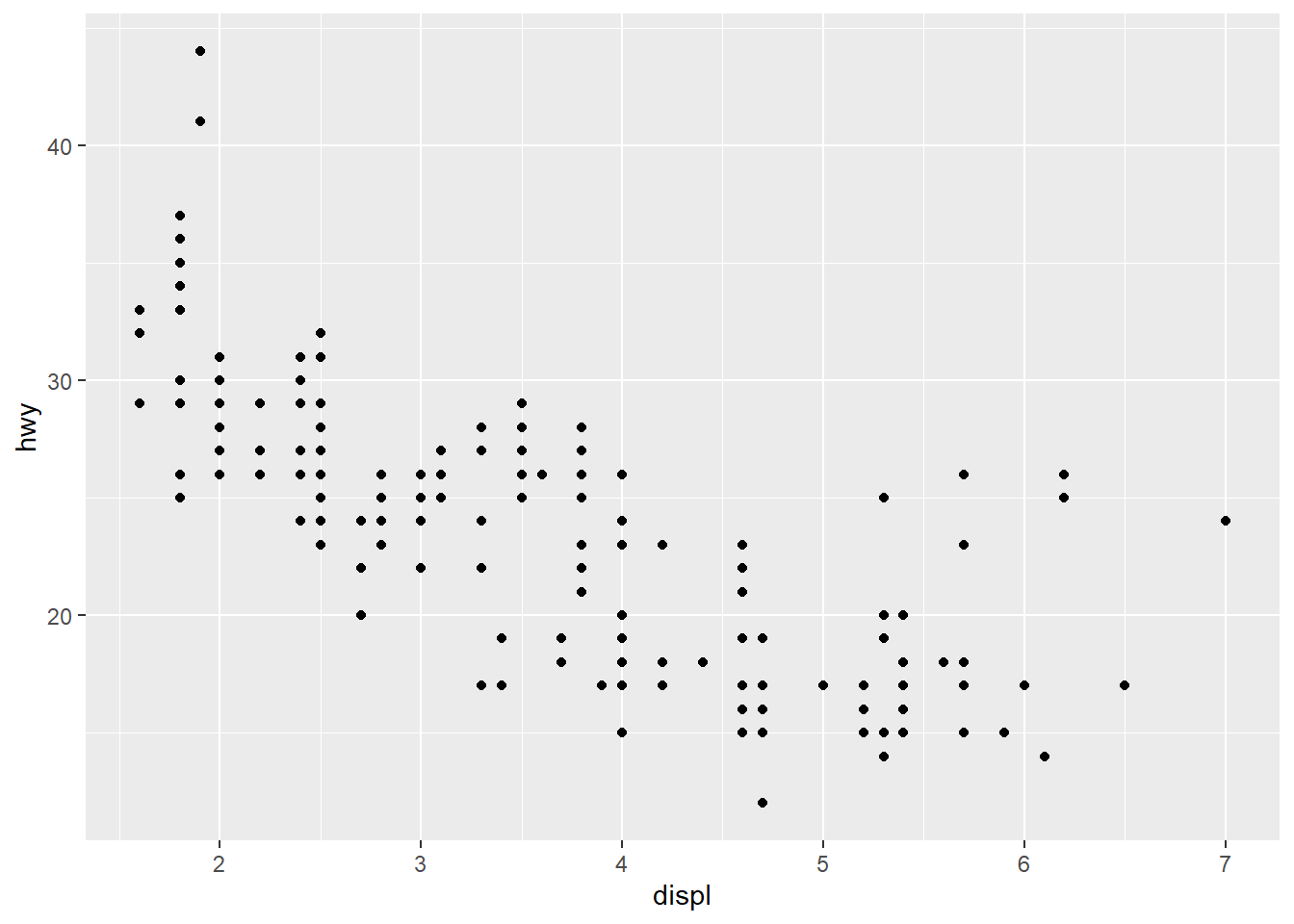

filter(mpg, cyl == 8)


    # A tibble: 70 x 11
       manufacturer model     displ  year   cyl trans  drv     cty   hwy fl    class
       <chr>        <chr>     <dbl> <int> <int> <chr>  <chr> <int> <int> <chr> <chr>
     1 audi         a6 quatt~   4.2  2008     8 auto(~ 4        16    23 p     mids~
     2 chevrolet    c1500 su~   5.3  2008     8 auto(~ r        14    20 r     suv  
     3 chevrolet    c1500 su~   5.3  2008     8 auto(~ r        11    15 e     suv  
     4 chevrolet    c1500 su~   5.3  2008     8 auto(~ r        14    20 r     suv  
     5 chevrolet    c1500 su~   5.7  1999     8 auto(~ r        13    17 r     suv  
     6 chevrolet    c1500 su~   6    2008     8 auto(~ r        12    17 r     suv  
     7 chevrolet    corvette    5.7  1999     8 manua~ r        16    26 p     2sea~
     8 chevrolet    corvette    5.7  1999     8 auto(~ r        15    23 p     2sea~
     9 chevrolet    corvette    6.2  2008     8 manua~ r        16    26 p     2sea~
    10 chevrolet    corvette    6.2  2008     8 auto(~ r        15    25 p     2sea~
    # ... with 60 more rows

filter(diamonds, carat > 3)


    # A tibble: 32 x 10
       carat cut     color clarity depth table price     x     y     z
       <dbl> <ord>   <ord> <ord>   <dbl> <dbl> <int> <dbl> <dbl> <dbl>
     1  3.01 Premium I     I1       62.7    58  8040  9.1   8.97  5.67
     2  3.11 Fair    J     I1       65.9    57  9823  9.15  9.02  5.98
     3  3.01 Premium F     I1       62.2    56  9925  9.24  9.13  5.73
     4  3.05 Premium E     I1       60.9    58 10453  9.26  9.25  5.66
     5  3.02 Fair    I     I1       65.2    56 10577  9.11  9.02  5.91
     6  3.01 Fair    H     I1       56.1    62 10761  9.54  9.38  5.31
     7  3.65 Fair    H     I1       67.1    53 11668  9.53  9.48  6.38
     8  3.24 Premium H     I1       62.1    58 12300  9.44  9.4   5.85
     9  3.22 Ideal   I     I1       62.6    55 12545  9.49  9.42  5.92
    10  3.5  Ideal   H     I1       62.8    57 12587  9.65  9.59  6.03
    # ... with 22 more rows

Press Alt + Shift + K. What happens? How can you get to the same place using the menus?

It opens the shortcuts popup page. You may close the page by pressing ESC.

To get there through the menus go to Tools -> Keyboard Shortcuts Help

sessionInfo()

R version 3.6.3 (2020-02-29)
Platform: x86_64-w64-mingw32/x64 (64-bit)
Running under: Windows 10 x64 (build 18363)

Matrix products: default

locale:
[1] LC_COLLATE=English_South Africa.1252  LC_CTYPE=English_South Africa.1252   
[3] LC_MONETARY=English_South Africa.1252 LC_NUMERIC=C                         
[5] LC_TIME=English_South Africa.1252    

attached base packages:
[1] stats     graphics  grDevices utils     datasets  methods   base     

other attached packages:
 [1] flair_0.0.2     forcats_0.5.0   stringr_1.4.0   dplyr_1.0.0    
 [5] purrr_0.3.4     readr_1.3.1     tidyr_1.1.0     tibble_3.0.3   
 [9] ggplot2_3.3.0   tidyverse_1.3.0 workflowr_1.6.2

loaded via a namespace (and not attached):
 [1] tidyselect_1.1.0 xfun_0.13        haven_2.2.0      lattice_0.20-38 
 [5] colorspace_1.4-1 vctrs_0.3.2      generics_0.0.2   htmltools_0.5.0 
 [9] yaml_2.2.1       utf8_1.1.4       rlang_0.4.7      later_1.0.0     
[13] pillar_1.4.6     withr_2.2.0      glue_1.4.1       DBI_1.1.0       
[17] dbplyr_1.4.3     modelr_0.1.6     readxl_1.3.1     lifecycle_0.2.0 
[21] munsell_0.5.0    gtable_0.3.0     cellranger_1.1.0 rvest_0.3.5     
[25] evaluate_0.14    labeling_0.3     knitr_1.28       httpuv_1.5.2    
[29] fansi_0.4.1      broom_0.5.6      Rcpp_1.0.4.6     promises_1.1.0  
[33] backports_1.1.6  scales_1.1.0     jsonlite_1.7.0   farver_2.0.3    
[37] fs_1.4.1         hms_0.5.3        digest_0.6.25    stringi_1.4.6   
[41] grid_3.6.3       rprojroot_1.3-2  cli_2.0.2        tools_3.6.3     
[45] magrittr_1.5     crayon_1.3.4     whisker_0.4      pkgconfig_2.0.3 
[49] ellipsis_0.3.1   xml2_1.3.2       reprex_0.3.0     lubridate_1.7.8 
[53] rstudioapi_0.11  assertthat_0.2.1 rmarkdown_2.4    httr_1.4.2      
[57] R6_2.4.1         nlme_3.1-144     git2r_0.26.1     compiler_3.6.3

Chapter 2 - Workflow basics

Vebash Naidoo

23/08/2020

Workflow …

Exercises