Chapter 14 - Pipes
Vebash Naidoo
18/10/2020
Last updated: 2020-11-09
Checks: 7 0
Knit directory: r4ds_book/
This reproducible R Markdown analysis was created with workflowr (version 1.6.2). The Checks tab describes the reproducibility checks that were applied when the results were created. The Past versions tab lists the development history.
Great! Since the R Markdown file has been committed to the Git repository, you know the exact version of the code that produced these results.
Great job! The global environment was empty. Objects defined in the global environment can affect the analysis in your R Markdown file in unknown ways. For reproduciblity it’s best to always run the code in an empty environment.
The command set.seed(20200814) was run prior to running the code in the R Markdown file. Setting a seed ensures that any results that rely on randomness, e.g. subsampling or permutations, are reproducible.
Great job! Recording the operating system, R version, and package versions is critical for reproducibility.
Nice! There were no cached chunks for this analysis, so you can be confident that you successfully produced the results during this run.
Great job! Using relative paths to the files within your workflowr project makes it easier to run your code on other machines.
Great! You are using Git for version control. Tracking code development and connecting the code version to the results is critical for reproducibility.
The results in this page were generated with repository version f3d860f. See the Past versions tab to see a history of the changes made to the R Markdown and HTML files.
Note that you need to be careful to ensure that all relevant files for the analysis have been committed to Git prior to generating the results (you can use wflow_publish or wflow_git_commit). workflowr only checks the R Markdown file, but you know if there are other scripts or data files that it depends on. Below is the status of the Git repository when the results were generated:
Ignored files:
    Ignored:    .Rproj.user/

Untracked files:
    Untracked:  analysis/images/
    Untracked:  code_snipp.txt
Note that any generated files, e.g. HTML, png, CSS, etc., are not included in this status report because it is ok for generated content to have uncommitted changes.
These are the previous versions of the repository in which changes were made to the R Markdown (analysis/ch14_pipes.Rmd) and HTML (docs/ch14_pipes.html) files. If you’ve configured a remote Git repository (see ?wflow_git_remote), click on the hyperlinks in the table below to view the files as they were in that past version.
| File | Version | Author | Date | Message |
|---|---|---|---|---|
| html | e423967 | sciencificity | 2020-11-08 | Build site. |
| html | 0d223fb | sciencificity | 2020-11-08 | Build site. |
| html | ecd1d8e | sciencificity | 2020-11-07 | Build site. |
| html | 274005c | sciencificity | 2020-11-06 | Build site. |
| html | 60e7ce2 | sciencificity | 2020-11-02 | Build site. |
| html | db5a796 | sciencificity | 2020-11-01 | Build site. |
| html | d8813e9 | sciencificity | 2020-11-01 | Build site. |
| html | bf15f3b | sciencificity | 2020-11-01 | Build site. |
| html | 0aef1b0 | sciencificity | 2020-10-31 | Build site. |
| html | bdc0881 | sciencificity | 2020-10-26 | Build site. |
| html | 8224544 | sciencificity | 2020-10-26 | Build site. |
| html | 2f8dcc0 | sciencificity | 2020-10-25 | Build site. |
| html | 61e2324 | sciencificity | 2020-10-25 | Build site. |
| html | 570c0bb | sciencificity | 2020-10-22 | Build site. |
| html | cfbefe6 | sciencificity | 2020-10-21 | Build site. |
| html | 4497db4 | sciencificity | 2020-10-18 | Build site. |
| Rmd | f81b11a | sciencificity | 2020-10-18 | added Chapter 14 and some of Chapter 8 |
options(scipen=10000)
library(palmerpenguins)
library(emo)
library(magrittr)
library(flair)
Pipes %>%
The ease of reading and writing code in R is a thing of beauty, and is made so due to the pipe! 💗 ❇️ 🆒.
Little bunny Foo Foo
Went hopping through the forest
Scooping up the field mice
And bopping them on the head
Intermediate Steps
foo_foo <-  little_bunny()
foo_foo1 <- hop(foo_foo, through = forest)
foo_foo2 <- scoop(foo_foo1, up = field_mice)
foo_foo3 <- bop(foo_foo2, on = head)- Main downside is that we need to name each intermediate step and with long data wrangling pipelines this can get tedious.
- The thought is that these extra copies also take up space, but they don’t. R cleverly handles that for us behind the scenes.
diamonds <- ggplot2::diamonds
diamonds2 <- diamonds %>%
  dplyr::mutate(price_per_carat = price / carat)

pryr::object_size(diamonds)  # gives memory occupied by all its args
3.46 MBpryr::object_size(diamonds2)3.89 MBpryr::object_size(diamonds, diamonds2) # collective size of both3.89 MBdiamonds and diamonds2 have 10 columns in common. These are shared by both objects.
If we modify any columns then the number of columns in common reduces. This is what happens below, and hence the shared size increases.
diamonds$carat[1] <- NA
pryr::object_size(diamonds)  # gives memory occupied by all its args
3.46 MBpryr::object_size(diamonds2)3.89 MBpryr::object_size(diamonds, diamonds2) # collective size of both4.32 MBOverwrite Original
foo_foo <-  little_bunny()
foo_foo <- hop(foo_foo, through = forest)
foo_foo <- scoop(foo_foo, up = field_mice)
foo_foo <- bop(foo_foo, on = head)- Debugging is hard. Need to re-run pipeline to figure out where the error lies.
- The common variable being overwritten hides whats happening at each step. E.g. Foo foo is a bunny who is hopping through the forest, and on her way she scoops up some field mice. A person reading your code will get confused as to what happened with Foo foo if they read long pipelines, or worse will think Foo foo can bop something on its head sometimes, can hop through a forest sometimes etc. I.e. it’s hard to keep track of what Foo foo is doing.
Function Composition
bop(
  scoop(
    hop(
      foo_foo,
      through = forest
    ),
    up = field_mice
  ),
  on = head
)- This way gets me the most, I struggle to keep track of what is happening when reading from the inside out, and I waste loads of paper drawing up pipelines like this to figure out what’s the end goal of the pipeline (sadly most other languages don’t have the
%>%)!
The pipe
foo_foo <- little_bunny()
foo_foo %>%
  hop(through = forest) %>%
  scoop(up = field_mice) %>%
  bop(on = head)
The authors remark that this is their favourite form, because it focusses on verbs, not nouns, and I am totally with them.
Foo foo hops through the forest, then scoops up field mice, then bops ’em on the head.
Behind the scenes magrittr creates a function with these steps and saves each in an intermediate object for us.
my_pipe <- function(.) {
  . <- hop(., through = forest)
  . <- scoop(., up = field_mice)
  bop(., on = head)
}
my_pipe(foo_foo)
The pipe does not work well for all functions though. Ones that use the current environment, functions using lazy evaluation like tryCatch().
Other useful pipe operators
Call a function for its side effects.
rnorm(100) %>%
  matrix(ncol = 2) %>%
  plot() %>%
  str()
NULLOur str() did not produce anything! 😭
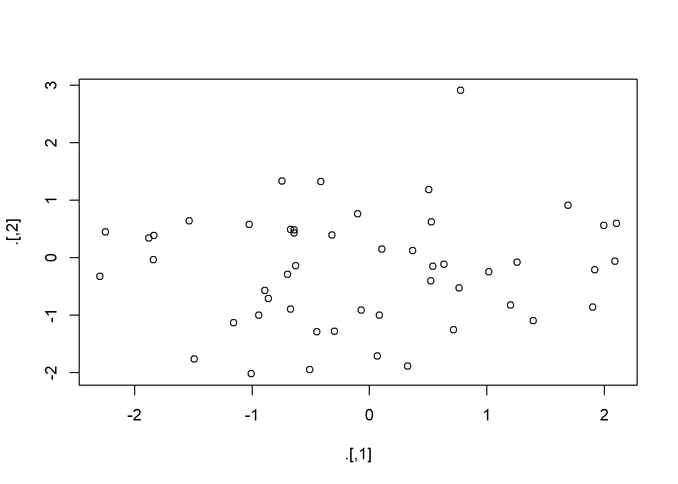
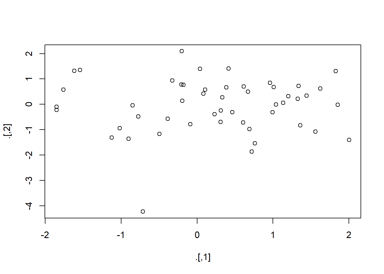
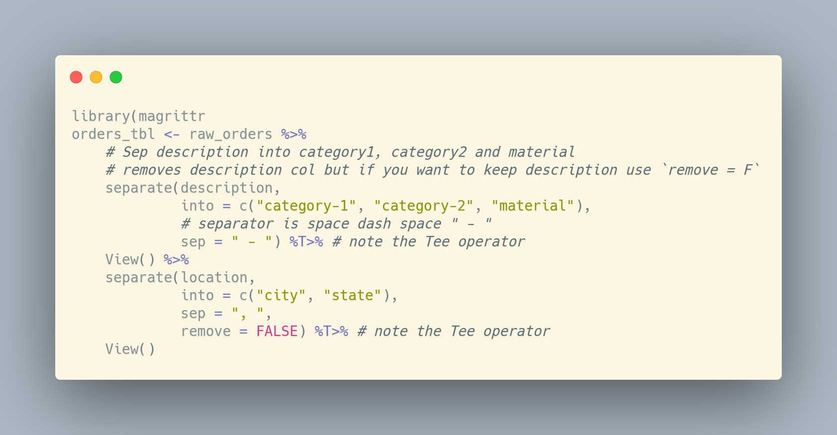
Enter the tee operator given by (%T>%). Things like print(), plot(), View() etc. do not return anything and when you use them in a pipeline it pipes nothing into the next step in the pipeline. A pipeline expects the result of the previous step to “replace” the first argument in the subsequent step though so this breaks the pipeline.
The %T>% does it’s job and sends the result of the previous pipe to the one after it’s side job function.
rnorm(100) %>%
  matrix(ncol = 2) %T>% # side job is to please plot
  plot() %>%
  str()
num [1:50, 1:2] 1.443 1.012 0.606 0.761 -0.849 ...The above takes matrix(rnorm(100, ncol = 2) and pipes it into str().


sessionInfo()R version 3.6.3 (2020-02-29)
Platform: x86_64-w64-mingw32/x64 (64-bit)
Running under: Windows 10 x64 (build 18363)
Matrix products: default
locale:
[1] LC_COLLATE=English_South Africa.1252 LC_CTYPE=English_South Africa.1252
[3] LC_MONETARY=English_South Africa.1252 LC_NUMERIC=C
[5] LC_TIME=English_South Africa.1252
attached base packages:
[1] stats graphics grDevices utils datasets methods base
other attached packages:
[1] flair_0.0.2 magrittr_1.5 emo_0.0.0.9000
[4] palmerpenguins_0.1.0 workflowr_1.6.2
loaded via a namespace (and not attached):
[1] Rcpp_1.0.4.6 pryr_0.1.4 pillar_1.4.6 compiler_3.6.3
[5] later_1.0.0 git2r_0.26.1 tools_3.6.3 digest_0.6.27
[9] gtable_0.3.0 lubridate_1.7.8 evaluate_0.14 lifecycle_0.2.0
[13] tibble_3.0.3 pkgconfig_2.0.3 rlang_0.4.8 rstudioapi_0.11
[17] yaml_2.2.1 xfun_0.13 dplyr_1.0.0 stringr_1.4.0
[21] knitr_1.28 generics_0.0.2 fs_1.5.0 vctrs_0.3.2
[25] tidyselect_1.1.0 grid_3.6.3 rprojroot_1.3-2 glue_1.4.2
[29] R6_2.4.1 rmarkdown_2.4 purrr_0.3.4 ggplot2_3.3.2
[33] whisker_0.4 codetools_0.2-16 scales_1.1.0 backports_1.1.6
[37] promises_1.1.0 ellipsis_0.3.1 htmltools_0.5.0 assertthat_0.2.1
[41] colorspace_1.4-1 httpuv_1.5.2 stringi_1.5.3 munsell_0.5.0
[45] crayon_1.3.4