Last updated: 2020-11-01

Checks: 7 0

Knit directory: r4ds_book/

This reproducible R Markdown analysis was created with workflowr (version 1.6.2). The Checks tab describes the reproducibility checks that were applied when the results were created. The Past versions tab lists the development history.

R Markdown file: up-to-date

Great! Since the R Markdown file has been committed to the Git repository, you know the exact version of the code that produced these results.

Environment: empty

Great job! The global environment was empty. Objects defined in the global environment can affect the analysis in your R Markdown file in unknown ways. For reproduciblity it’s best to always run the code in an empty environment.

Seed: set.seed(20200814)

The command set.seed(20200814) was run prior to running the code in the R Markdown file. Setting a seed ensures that any results that rely on randomness, e.g. subsampling or permutations, are reproducible.

Session information: recorded

Great job! Recording the operating system, R version, and package versions is critical for reproducibility.

Cache: none

Nice! There were no cached chunks for this analysis, so you can be confident that you successfully produced the results during this run.

File paths: relative

Great job! Using relative paths to the files within your workflowr project makes it easier to run your code on other machines.

Repository version: 2cd3513

Great! You are using Git for version control. Tracking code development and connecting the code version to the results is critical for reproducibility.

The results in this page were generated with repository version 2cd3513. See the Past versions tab to see a history of the changes made to the R Markdown and HTML files.

Note that you need to be careful to ensure that all relevant files for the analysis have been committed to Git prior to generating the results (you can use wflow_publish or wflow_git_commit). workflowr only checks the R Markdown file, but you know if there are other scripts or data files that it depends on. Below is the status of the Git repository when the results were generated:


Ignored files:
    Ignored:    .Rproj.user/

Untracked files:
    Untracked:  analysis/images/
    Untracked:  code_snipp.txt

Note that any generated files, e.g. HTML, png, CSS, etc., are not included in this status report because it is ok for generated content to have uncommitted changes.

These are the previous versions of the repository in which changes were made to the R Markdown (analysis/ch10_relations_dplyr.Rmd) and HTML (docs/ch10_relations_dplyr.html) files. If you’ve configured a remote Git repository (see ?wflow_git_remote), click on the hyperlinks in the table below to view the files as they were in that past version.

File	Version	Author	Date	Message
html	d8813e9	sciencificity	2020-11-01	Build site.
html	bf15f3b	sciencificity	2020-11-01	Build site.
html	0aef1b0	sciencificity	2020-10-31	Build site.
Rmd	72ad7d9	sciencificity	2020-10-31	added ch10

Relational Data

Click on the tab buttons below for each section

Main types of joins

Mutating joins, which add new variables to one data frame from matching observations in another.
Filtering joins, which filter observations from one data frame based on whether or not they match an observation in the other table.
Set operations, which treat observations as if they were set elements.

Dataset

These are the datasets we will be using to learn about joins which come from the nycflights13 package.

airlines lets you look up the full carrier name from its abbreviated code:

airlines
#> # A tibble: 16 x 2
#>    carrier name                       
#>    <chr>   <chr>                      
#>  1 9E      Endeavor Air Inc.          
#>  2 AA      American Airlines Inc.     
#>  3 AS      Alaska Airlines Inc.       
#>  4 B6      JetBlue Airways            
#>  5 DL      Delta Air Lines Inc.       
#>  6 EV      ExpressJet Airlines Inc.   
#>  7 F9      Frontier Airlines Inc.     
#>  8 FL      AirTran Airways Corporation
#>  9 HA      Hawaiian Airlines Inc.     
#> 10 MQ      Envoy Air                  
#> 11 OO      SkyWest Airlines Inc.      
#> 12 UA      United Air Lines Inc.      
#> 13 US      US Airways Inc.            
#> 14 VX      Virgin America             
#> 15 WN      Southwest Airlines Co.     
#> 16 YV      Mesa Airlines Inc.

airports gives information about each airport, identified by the faa airport code:

airports
#> # A tibble: 1,458 x 8
#>    faa   name                       lat    lon   alt    tz dst   tzone          
#>    <chr> <chr>                    <dbl>  <dbl> <dbl> <dbl> <chr> <chr>          
#>  1 04G   Lansdowne Airport         41.1  -80.6  1044    -5 A     America/New_Yo~
#>  2 06A   Moton Field Municipal A~  32.5  -85.7   264    -6 A     America/Chicago
#>  3 06C   Schaumburg Regional       42.0  -88.1   801    -6 A     America/Chicago
#>  4 06N   Randall Airport           41.4  -74.4   523    -5 A     America/New_Yo~
#>  5 09J   Jekyll Island Airport     31.1  -81.4    11    -5 A     America/New_Yo~
#>  6 0A9   Elizabethton Municipal ~  36.4  -82.2  1593    -5 A     America/New_Yo~
#>  7 0G6   Williams County Airport   41.5  -84.5   730    -5 A     America/New_Yo~
#>  8 0G7   Finger Lakes Regional A~  42.9  -76.8   492    -5 A     America/New_Yo~
#>  9 0P2   Shoestring Aviation Air~  39.8  -76.6  1000    -5 U     America/New_Yo~
#> 10 0S9   Jefferson County Intl     48.1 -123.    108    -8 A     America/Los_An~
#> # ... with 1,448 more rows

planes gives information about each plane, identified by its tailnum:

planes
#> # A tibble: 3,322 x 9
#>    tailnum  year type          manufacturer   model  engines seats speed engine 
#>    <chr>   <int> <chr>         <chr>          <chr>    <int> <int> <int> <chr>  
#>  1 N10156   2004 Fixed wing m~ EMBRAER        EMB-1~       2    55    NA Turbo-~
#>  2 N102UW   1998 Fixed wing m~ AIRBUS INDUST~ A320-~       2   182    NA Turbo-~
#>  3 N103US   1999 Fixed wing m~ AIRBUS INDUST~ A320-~       2   182    NA Turbo-~
#>  4 N104UW   1999 Fixed wing m~ AIRBUS INDUST~ A320-~       2   182    NA Turbo-~
#>  5 N10575   2002 Fixed wing m~ EMBRAER        EMB-1~       2    55    NA Turbo-~
#>  6 N105UW   1999 Fixed wing m~ AIRBUS INDUST~ A320-~       2   182    NA Turbo-~
#>  7 N107US   1999 Fixed wing m~ AIRBUS INDUST~ A320-~       2   182    NA Turbo-~
#>  8 N108UW   1999 Fixed wing m~ AIRBUS INDUST~ A320-~       2   182    NA Turbo-~
#>  9 N109UW   1999 Fixed wing m~ AIRBUS INDUST~ A320-~       2   182    NA Turbo-~
#> 10 N110UW   1999 Fixed wing m~ AIRBUS INDUST~ A320-~       2   182    NA Turbo-~
#> # ... with 3,312 more rows

weather gives the weather at each NYC airport for each hour:

weather
#> # A tibble: 26,115 x 15
#>    origin  year month   day  hour  temp  dewp humid wind_dir wind_speed
#>    <chr>  <int> <int> <int> <int> <dbl> <dbl> <dbl>    <dbl>      <dbl>
#>  1 EWR     2013     1     1     1  39.0  26.1  59.4      270      10.4 
#>  2 EWR     2013     1     1     2  39.0  27.0  61.6      250       8.06
#>  3 EWR     2013     1     1     3  39.0  28.0  64.4      240      11.5 
#>  4 EWR     2013     1     1     4  39.9  28.0  62.2      250      12.7 
#>  5 EWR     2013     1     1     5  39.0  28.0  64.4      260      12.7 
#>  6 EWR     2013     1     1     6  37.9  28.0  67.2      240      11.5 
#>  7 EWR     2013     1     1     7  39.0  28.0  64.4      240      15.0 
#>  8 EWR     2013     1     1     8  39.9  28.0  62.2      250      10.4 
#>  9 EWR     2013     1     1     9  39.9  28.0  62.2      260      15.0 
#> 10 EWR     2013     1     1    10  41    28.0  59.6      260      13.8 
#> # ... with 26,105 more rows, and 5 more variables: wind_gust <dbl>,
#> #   precip <dbl>, pressure <dbl>, visib <dbl>, time_hour <dttm>

flights gives the flights departing a NYC airport:

flights
#> # A tibble: 336,776 x 19
#>     year month   day dep_time sched_dep_time dep_delay arr_time sched_arr_time
#>    <int> <int> <int>    <int>          <int>     <dbl>    <int>          <int>
#>  1  2013     1     1      517            515         2      830            819
#>  2  2013     1     1      533            529         4      850            830
#>  3  2013     1     1      542            540         2      923            850
#>  4  2013     1     1      544            545        -1     1004           1022
#>  5  2013     1     1      554            600        -6      812            837
#>  6  2013     1     1      554            558        -4      740            728
#>  7  2013     1     1      555            600        -5      913            854
#>  8  2013     1     1      557            600        -3      709            723
#>  9  2013     1     1      557            600        -3      838            846
#> 10  2013     1     1      558            600        -2      753            745
#> # ... with 336,766 more rows, and 11 more variables: arr_delay <dbl>,
#> #   carrier <chr>, flight <int>, tailnum <chr>, origin <chr>, dest <chr>,
#> #   air_time <dbl>, distance <dbl>, hour <dbl>, minute <dbl>, time_hour <dttm>

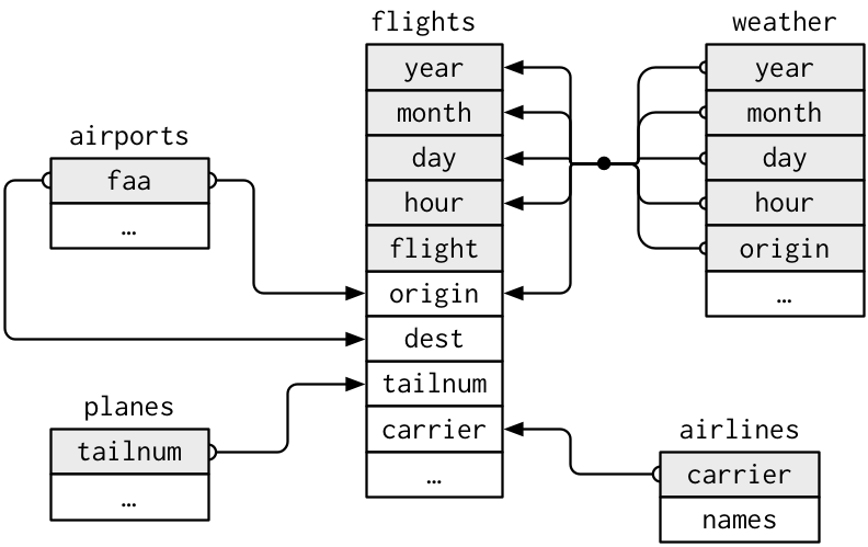
ERD — Enterprise Relation Diagram from R4DS

For nycflights13:

flights connects to planes via a single variable, tailnum.
flights connects to airlines through the carrier variable.
flights connects to airports in two ways: via the origin and dest variables.
flights connects to weather via origin (the location), and year, month, day and hour (the time).

Exercises

Imagine you wanted to draw (approximately) the route each plane flies from its origin to its destination. What variables would you need? What tables would you need to combine?

We would need the origin and dest from flights and the lat and lon for each origin / dest from airports.
I forgot to draw the relationship between weather and airports. What is the relationship and how should it appear in the diagram?

weather has origin, and airports has faa. These could be joined to get all weather conditions for each day and each hour in the dataset.
weather only contains information for the origin (NYC) airports. If it contained weather records for all airports in the USA, what additional relation would it define with flights?

There would be a relation with dest.
We know that some days of the year are “special”, and fewer people than usual fly on them. How might you represent that data as a data frame? What would be the primary keys of that table? How would it connect to the existing tables?

I would have a table called holidays and it would have a year, month and day variable that can be used to connect to flights, and weather.

Keys

A table has a name, a column too has a name.
Rows however don’t have names, and need a way to be identified. This is done through a primary key. A primary key identifies a single row in a table. It is unique since no two rows can have the same primary key. It may be simple (a single column serves as the primary key) or composite (multiple columns serve as the primary key).
For example, planes$tailnum is a primary key because it uniquely identifies each plane in the planes table.
Data is spread among several columns. A foreign key allows you to associate the different tables you have. A foreign key is either a single column or multiple columns that reference values in some other table.
For example, flights$tailnum is a foreign key because it appears in the flights table where it matches each flight to a unique plane in the planes table.
A variable can be both a primary key and a foreign key. For example, origin is part of the weather primary key, and is also a foreign key for the airports table.

airlines %>% 
  count(carrier) %>% 
  filter(n > 1)
#> # A tibble: 0 x 2
#> # ... with 2 variables: carrier , n 

airports %>% 
  count(faa) %>% 
  filter(n > 1)
#> # A tibble: 0 x 2
#> # ... with 2 variables: faa , n 

planes %>% 
  count(tailnum) %>% 
  filter(n > 1)
#> # A tibble: 0 x 2
#> # ... with 2 variables: tailnum , n 

weather %>% 
  count(year, month, day, hour, origin) %>% 
  filter(n > 1)  
#> # A tibble: 3 x 6
#>    year month   day  hour origin     n
#>         
#> 1  2013    11     3     1 EWR        2
#> 2  2013    11     3     1 JFK        2
#> 3  2013    11     3     1 LGA        2
  
weather %>% 
  filter(year == 2013,
         month == 11,
         day == 3,
         hour == 1) %>% 
  print(width = Inf)
#> # A tibble: 6 x 15
#>   origin  year month   day  hour  temp  dewp humid wind_dir wind_speed wind_gust
#>                          
#> 1 EWR     2013    11     3     1  52.0  39.0  61.2      310       6.90        NA
#> 2 EWR     2013    11     3     1  50    39.0  65.8      290       5.75        NA
#> 3 JFK     2013    11     3     1  54.0  37.9  54.5      320       9.21        NA
#> 4 JFK     2013    11     3     1  52.0  37.9  58.6      310       6.90        NA
#> 5 LGA     2013    11     3     1  55.0  39.0  54.7      330       9.21        NA
#> 6 LGA     2013    11     3     1  54.0  39.9  58.9      310       8.06        NA
#>   precip pressure visib time_hour          
#>                       
#> 1      0    1010.    10 2013-11-03 01:00:00
#> 2      0    1010.    10 2013-11-03 01:00:00
#> 3      0    1010.    10 2013-11-03 01:00:00
#> 4      0    1010.    10 2013-11-03 01:00:00
#> 5      0    1009.    10 2013-11-03 01:00:00
#> 6      0    1010.    10 2013-11-03 01:00:00

weather %>% 
  filter(year == 2013,
         month == 11,
         day == 3,
         hour == 1) %>% 
  mutate(lag = lag(time_hour),
         lead = lead(time_hour),
         diff = time_hour - lag) %>% 
  print(width = Inf)
#> # A tibble: 6 x 18
#>   origin  year month   day  hour  temp  dewp humid wind_dir wind_speed wind_gust
#>                          
#> 1 EWR     2013    11     3     1  52.0  39.0  61.2      310       6.90        NA
#> 2 EWR     2013    11     3     1  50    39.0  65.8      290       5.75        NA
#> 3 JFK     2013    11     3     1  54.0  37.9  54.5      320       9.21        NA
#> 4 JFK     2013    11     3     1  52.0  37.9  58.6      310       6.90        NA
#> 5 LGA     2013    11     3     1  55.0  39.0  54.7      330       9.21        NA
#> 6 LGA     2013    11     3     1  54.0  39.9  58.9      310       8.06        NA
#>   precip pressure visib time_hour           lag                
#>                                     
#> 1      0    1010.    10 2013-11-03 01:00:00 NA                 
#> 2      0    1010.    10 2013-11-03 01:00:00 2013-11-03 01:00:00
#> 3      0    1010.    10 2013-11-03 01:00:00 2013-11-03 01:00:00
#> 4      0    1010.    10 2013-11-03 01:00:00 2013-11-03 01:00:00
#> 5      0    1009.    10 2013-11-03 01:00:00 2013-11-03 01:00:00
#> 6      0    1010.    10 2013-11-03 01:00:00 2013-11-03 01:00:00
#>   lead                diff    
#>                   
#> 1 2013-11-03 01:00:00 NA hours
#> 2 2013-11-03 01:00:00  1 hours
#> 3 2013-11-03 01:00:00 -1 hours
#> 4 2013-11-03 01:00:00  1 hours
#> 5 2013-11-03 01:00:00 -1 hours
#> 6 NA                   1 hours
  

weather %>% 
  count(year, month, day, hour, origin, time_hour) %>% 
  filter(n > 1)
#> # A tibble: 0 x 7
#> # ... with 7 variables: year , month , day , hour ,
#> #   origin , time_hour , n 

weather %>% 
  print(width = Inf)
#> # A tibble: 26,115 x 15
#>    origin  year month   day  hour  temp  dewp humid wind_dir wind_speed
#>                      
#>  1 EWR     2013     1     1     1  39.0  26.1  59.4      270      10.4 
#>  2 EWR     2013     1     1     2  39.0  27.0  61.6      250       8.06
#>  3 EWR     2013     1     1     3  39.0  28.0  64.4      240      11.5 
#>  4 EWR     2013     1     1     4  39.9  28.0  62.2      250      12.7 
#>  5 EWR     2013     1     1     5  39.0  28.0  64.4      260      12.7 
#>  6 EWR     2013     1     1     6  37.9  28.0  67.2      240      11.5 
#>  7 EWR     2013     1     1     7  39.0  28.0  64.4      240      15.0 
#>  8 EWR     2013     1     1     8  39.9  28.0  62.2      250      10.4 
#>  9 EWR     2013     1     1     9  39.9  28.0  62.2      260      15.0 
#> 10 EWR     2013     1     1    10  41    28.0  59.6      260      13.8 
#>    wind_gust precip pressure visib time_hour          
#>                             
#>  1        NA      0    1012     10 2013-01-01 01:00:00
#>  2        NA      0    1012.    10 2013-01-01 02:00:00
#>  3        NA      0    1012.    10 2013-01-01 03:00:00
#>  4        NA      0    1012.    10 2013-01-01 04:00:00
#>  5        NA      0    1012.    10 2013-01-01 05:00:00
#>  6        NA      0    1012.    10 2013-01-01 06:00:00
#>  7        NA      0    1012.    10 2013-01-01 07:00:00
#>  8        NA      0    1012.    10 2013-01-01 08:00:00
#>  9        NA      0    1013.    10 2013-01-01 09:00:00
#> 10        NA      0    1012.    10 2013-01-01 10:00:00
#> # ... with 26,105 more rows

flights %>% 
  count(year, month, day, hour, 
        origin, dest, carrier,
        tailnum) %>% 
  filter(n > 1)
#> # A tibble: 13 x 9
#>     year month   day  hour origin dest  carrier tailnum     n
#>                 
#>  1  2013     1     7     6 LGA    ORD   AA      N3CYAA      2
#>  2  2013     2     8    16 EWR    ORD   UA              2
#>  3  2013     2     9     6 EWR    CLT   US              2
#>  4  2013     2     9     6 LGA    CLT   US              2
#>  5  2013     2     9     6 LGA    DFW   AA              2
#>  6  2013     2     9     6 LGA    ORD   AA              2
#>  7  2013     2     9     7 LGA    MIA   AA              2
#>  8  2013     3    19     7 LGA    ORD   AA      N4XMAA      2
#>  9  2013     6    12    18 LGA    ORD   UA              2
#> 10  2013     7     6    15 EWR    SFO   UA              2
#> 11  2013     9     2    17 LGA    ORD   UA              2
#> 12  2013     9    12    17 LGA    ORD   UA              2
#> 13  2013    11    25     6 LGA    DFW   AA              2

# Let's have a look at a few
flights %>% 
  filter(year == 2013, month == 1, day == 7, hour == "6",
         origin == "LGA", dest == "ORD",
         carrier == "AA", tailnum == "N3CYAA") %>% 
  print(width = Inf)
#> # A tibble: 2 x 19
#>    year month   day dep_time sched_dep_time dep_delay arr_time sched_arr_time
#>                                      
#> 1  2013     1     7      634            630         4      758            810
#> 2  2013     1     7       NA            600        NA       NA            745
#>   arr_delay carrier flight tailnum origin dest  air_time distance  hour minute
#>                             
#> 1       -12 AA         303 N3CYAA  LGA    ORD        116      733     6     30
#> 2        NA AA         301 N3CYAA  LGA    ORD         NA      733     6      0
#>   time_hour          
#>                
#> 1 2013-01-07 06:00:00
#> 2 2013-01-07 06:00:00

flights %>% 
  count(year, month, day, hour, 
        origin, dest, carrier,
        tailnum, flight) %>% 
  filter(n > 1)
#> # A tibble: 0 x 10
#> # ... with 10 variables: year , month , day , hour ,
#> #   origin , dest , carrier , tailnum , flight ,
#> #   n

When even a combination of columns does not seem to identify an observation you may add your own primary key. The best is to use mutate with row_number(). This is called a surrogate key.

Exercises

Add a surrogate key to flights.

(flights_pk <- flights %>% 
  mutate(pk = row_number())) %T>%
   print(width = Inf)
#> # A tibble: 336,776 x 20
#>     year month   day dep_time sched_dep_time dep_delay arr_time sched_arr_time
#>    <int> <int> <int>    <int>          <int>     <dbl>    <int>          <int>
#>  1  2013     1     1      517            515         2      830            819
#>  2  2013     1     1      533            529         4      850            830
#>  3  2013     1     1      542            540         2      923            850
#>  4  2013     1     1      544            545        -1     1004           1022
#>  5  2013     1     1      554            600        -6      812            837
#>  6  2013     1     1      554            558        -4      740            728
#>  7  2013     1     1      555            600        -5      913            854
#>  8  2013     1     1      557            600        -3      709            723
#>  9  2013     1     1      557            600        -3      838            846
#> 10  2013     1     1      558            600        -2      753            745
#>    arr_delay carrier flight tailnum origin dest  air_time distance  hour minute
#>        <dbl> <chr>    <int> <chr>   <chr>  <chr>    <dbl>    <dbl> <dbl>  <dbl>
#>  1        11 UA        1545 N14228  EWR    IAH        227     1400     5     15
#>  2        20 UA        1714 N24211  LGA    IAH        227     1416     5     29
#>  3        33 AA        1141 N619AA  JFK    MIA        160     1089     5     40
#>  4       -18 B6         725 N804JB  JFK    BQN        183     1576     5     45
#>  5       -25 DL         461 N668DN  LGA    ATL        116      762     6      0
#>  6        12 UA        1696 N39463  EWR    ORD        150      719     5     58
#>  7        19 B6         507 N516JB  EWR    FLL        158     1065     6      0
#>  8       -14 EV        5708 N829AS  LGA    IAD         53      229     6      0
#>  9        -8 B6          79 N593JB  JFK    MCO        140      944     6      0
#> 10         8 AA         301 N3ALAA  LGA    ORD        138      733     6      0
#>    time_hour              pk
#>    <dttm>              <int>
#>  1 2013-01-01 05:00:00     1
#>  2 2013-01-01 05:00:00     2
#>  3 2013-01-01 05:00:00     3
#>  4 2013-01-01 05:00:00     4
#>  5 2013-01-01 06:00:00     5
#>  6 2013-01-01 05:00:00     6
#>  7 2013-01-01 06:00:00     7
#>  8 2013-01-01 06:00:00     8
#>  9 2013-01-01 06:00:00     9
#> 10 2013-01-01 06:00:00    10
#> # ... with 336,766 more rows
#> # A tibble: 336,776 x 20
#>     year month   day dep_time sched_dep_time dep_delay arr_time sched_arr_time
#>    <int> <int> <int>    <int>          <int>     <dbl>    <int>          <int>
#>  1  2013     1     1      517            515         2      830            819
#>  2  2013     1     1      533            529         4      850            830
#>  3  2013     1     1      542            540         2      923            850
#>  4  2013     1     1      544            545        -1     1004           1022
#>  5  2013     1     1      554            600        -6      812            837
#>  6  2013     1     1      554            558        -4      740            728
#>  7  2013     1     1      555            600        -5      913            854
#>  8  2013     1     1      557            600        -3      709            723
#>  9  2013     1     1      557            600        -3      838            846
#> 10  2013     1     1      558            600        -2      753            745
#> # ... with 336,766 more rows, and 12 more variables: arr_delay <dbl>,
#> #   carrier <chr>, flight <int>, tailnum <chr>, origin <chr>, dest <chr>,
#> #   air_time <dbl>, distance <dbl>, hour <dbl>, minute <dbl>, time_hour <dttm>,
#> #   pk <int>

Identify the keys in the following datasets

Lahman::Batting

Wondering how to figure out what datasets are available to you to use?

Call data(package = 'XXX') to get a listing.

data(package = "Lahman") %>% 
  print()

The above produces a list like this 🔻:

Data in a package Lahman — data(package = ‘name_of_pkg’)

data("Batting", package = "Lahman")
# data("Salaries", package = "Lahman")
# data("People", package = "Lahman")

as_tibble(Batting) %>% 
# first try
count(playerID, yearID, teamID) %>% 
filter(n > 1)
#> # A tibble: 70 x 4
#>    playerID  yearID teamID     n
#>    <chr>      <int> <fct>  <int>
#>  1 alyeabr01   1972 OAK        2
#>  2 anderjo01   1898 BRO        2
#>  3 baldwja01   2005 BAL        2
#>  4 behrmha01   1947 BRO        2
#>  5 chouife01   1914 BRF        3
#>  6 clarkje02   2003 TEX        2
#>  7 clarkni01   1905 CLE        2
#>  8 cranddo01   1913 NY1        2
#>  9 cranesa01   1890 NY1        2
#> 10 donahpa01   1910 PHA        2
#> # ... with 60 more rows

as_tibble(Batting) %>%  
  # let's have a look at one to see what else
  # differentiates it
  filter(playerID == "alyeabr01",
        yearID == 1972,
        teamID == "OAK")
#> # A tibble: 2 x 22
#>   playerID yearID stint teamID lgID      G    AB     R     H   X2B   X3B    HR
#>   <chr>     <int> <int> <fct>  <fct> <int> <int> <int> <int> <int> <int> <int>
#> 1 alyeabr~   1972     1 OAK    AL       10    13     1     3     1     0     0
#> 2 alyeabr~   1972     3 OAK    AL       10    18     2     3     0     0     1
#> # ... with 10 more variables: RBI <int>, SB <int>, CS <int>, BB <int>,
#> #   SO <int>, IBB <int>, HBP <int>, SH <int>, SF <int>, GIDP <int>

as_tibble(Batting) %>% 
  count(playerID, yearID, teamID, stint) %>% 
  filter(n > 1)
#> # A tibble: 0 x 5
#> # ... with 5 variables: playerID <chr>, yearID <int>, teamID <fct>,
#> #   stint <int>, n <int>

Looks like the key is playerID, yearID, teamID and stint.

babynames::babynames

data(babynames, package = "babynames")
class(babynames)
#> [1] "tbl_df"     "tbl"        "data.frame"
babynames
#> # A tibble: 1,924,665 x 5
#>     year sex   name          n   prop
#>    <dbl> <chr> <chr>     <int>  <dbl>
#>  1  1880 F     Mary       7065 0.0724
#>  2  1880 F     Anna       2604 0.0267
#>  3  1880 F     Emma       2003 0.0205
#>  4  1880 F     Elizabeth  1939 0.0199
#>  5  1880 F     Minnie     1746 0.0179
#>  6  1880 F     Margaret   1578 0.0162
#>  7  1880 F     Ida        1472 0.0151
#>  8  1880 F     Alice      1414 0.0145
#>  9  1880 F     Bertha     1320 0.0135
#> 10  1880 F     Sarah      1288 0.0132
#> # ... with 1,924,655 more rows
babynames %>% 
  # n is in the columns so we need to name our variable
  # something else
  dplyr::count(year, sex, name,
              name = "count",
  # without the wt = 1, it was using n as a weight in count                  
  # Using `n` as weighting variable
  # i Quiet this message with `wt = n` or count rows with `wt = 1`
              wt = 1) %>% 
  filter(count > 1)
#> # A tibble: 0 x 4
#> # ... with 4 variables: year <dbl>, sex <chr>, name <chr>, count <dbl>

babynames %>% 
  group_by(year, sex, name) %>% 
  summarise(nn = n())
#> # A tibble: 1,924,665 x 4
#> # Groups:   year, sex [276]
#>     year sex   name        nn
#>    <dbl> <chr> <chr>    <int>
#>  1  1880 F     Abbie        1
#>  2  1880 F     Abby         1
#>  3  1880 F     Abigail      1
#>  4  1880 F     Ada          1
#>  5  1880 F     Adah         1
#>  6  1880 F     Adaline      1
#>  7  1880 F     Adda         1
#>  8  1880 F     Addie        1
#>  9  1880 F     Adela        1
#> 10  1880 F     Adelaide     1
#> # ... with 1,924,655 more rows

babynames %>% 
  # confirming there is only one row for each
  filter(year == 1880, 
         sex == 'F',
         name == 'Abby' | name == "Adda")
#> # A tibble: 2 x 5
#>    year sex   name      n      prop
#>   <dbl> <chr> <chr> <int>     <dbl>
#> 1  1880 F     Adda     14 0.000143 
#> 2  1880 F     Abby      6 0.0000615

Looks like the key is year, sex, name. So, we had some issues here, since the dataset had an n variable in it. The count() / tally() function uses n as a weighting variable.

To fix this we need to:

explicitly name the output variable something other than n
add a wt = 1 to not tally up the n.

Let’s see this with the example tribble in the help docs.

First as it should be:

# use the `wt` argument to perform a weighted count. This is useful
# when the data has already been aggregated once
(df <- tribble(
  ~name,    ~gender,   ~runs,
  "Max",    "male",       10,
  "Sandra", "female",      1,
  "Susan",  "female",      4
))
#> # A tibble: 3 x 3
#>   name   gender  runs
#>   <chr>  <chr>  <dbl>
#> 1 Max    male      10
#> 2 Sandra female     1
#> 3 Susan  female     4
# counts rows:
df %>% count(gender)
#> # A tibble: 2 x 2
#>   gender     n
#>   <chr>  <int>
#> 1 female     2
#> 2 male       1
# counts runs:
df %>% count(gender, wt = runs)
#> # A tibble: 2 x 2
#>   gender     n
#>   <chr>  <dbl>
#> 1 female     5
#> 2 male      10

Now let’s rename runs to n, and we see the difference:

# use the `wt` argument to perform a weighted count. This is useful
# when the data has already been aggregated once
(df <- tribble(
  ~name,    ~gender,      ~n,
  "Max",    "male",       10,
  "Sandra", "female",      1,
  "Susan",  "female",      4
))
#> # A tibble: 3 x 3
#>   name   gender     n
#>   <chr>  <chr>  <dbl>
#> 1 Max    male      10
#> 2 Sandra female     1
#> 3 Susan  female     4
# counts rows:
df %>% count(gender) # weight(wt) = n implicit
#> # A tibble: 2 x 2
#>   gender     n
#>   <chr>  <dbl>
#> 1 female     5
#> 2 male      10

Adding a new name and a wt = 1 we should get the original output as when we used the variable named runs. Here it shows female as 1 which is not correct. 🙀

# use the `wt` argument to perform a weighted count. This is useful
# when the data has already been aggregated once
(df <- tribble(
  ~name,    ~gender,      ~n,
  "Max",    "male",       10,
  "Sandra", "female",      1,
  "Susan",  'female',      4
))
#> # A tibble: 3 x 3
#>   name   gender     n
#>   <chr>  <chr>  <dbl>
#> 1 Max    male      10
#> 2 Sandra female     1
#> 3 Susan  female     4
# counts rows:
df %>% count(gender, 
             name = "count", 
             wt = 1
             )
#> # A tibble: 2 x 2
#>   gender count
#>   <chr>  <dbl>
#> 1 female     1
#> 2 male       1
# counts n's:
df %>% count(gender, name = "count", wt = n)
#> # A tibble: 2 x 2
#>   gender count
#>   <chr>  <dbl>
#> 1 female     5
#> 2 male      10

I am unsure what is really going on above, as I expected female = 2, but I don’t have time to investigate. It does work for the babynames case so this may be some other anomaly - maybe convert to a factor and see?

nasaweather::atmos

data("atmos", package = "nasaweather")

atmos %>% 
  count(lat, long, year, month) %>% 
  filter(n > 1)
#> # A tibble: 0 x 5
#> # ... with 5 variables: lat <dbl>, long <dbl>, year <int>, month <int>, n <int>

Looks like the key is lat, long, year and month.

fueleconomy::vehicles

fueleconomy::vehicles %>% 
  count(id) %>% 
  filter(n > 1)
#> # A tibble: 0 x 2
#> # ... with 2 variables: id <dbl>, n <int>

Looks like the key is id.

ggplot2::diamonds

ggplot2::diamonds %>% 
  count(carat, cut, color, clarity, price, depth, table, x, y, z) %>% 
  filter(n > 1)
#> # A tibble: 143 x 11
#>    carat cut       color clarity price depth table     x     y     z     n
#>    <dbl> <ord>     <ord> <ord>   <int> <dbl> <dbl> <dbl> <dbl> <dbl> <int>
#>  1  0.3  Good      J     VS1       394  63.4    57  4.23  4.26  2.69     2
#>  2  0.3  Very Good G     VS2       526  63      55  4.29  4.31  2.71     2
#>  3  0.3  Very Good J     VS1       506  63.4    57  4.26  4.23  2.69     2
#>  4  0.3  Premium   D     SI1       709  62.2    58  4.31  4.28  2.67     2
#>  5  0.3  Ideal     G     VS2       675  63      55  4.31  4.29  2.71     2
#>  6  0.3  Ideal     G     IF        863  62.1    55  4.32  4.35  2.69     2
#>  7  0.3  Ideal     H     SI1       450  62.2    57  4.26  4.29  2.66     2
#>  8  0.3  Ideal     H     SI1       450  62.2    57  4.27  4.28  2.66     2
#>  9  0.31 Good      D     SI1       571  63.5    56  4.29  4.31  2.73     2
#> 10  0.31 Very Good D     SI1       732  63.5    56  4.31  4.29  2.73     2
#> # ... with 133 more rows

There is not a clear key for diamonds so here we would create one using a surrogate key via a mutate and row_number().

Draw a diagram illustrating the connections between the Batting, People, and Salaries tables in the Lahman package. Draw another diagram that shows the relationship between People, Managers, AwardsManagers.

How would you characterise the relationship between the Batting, Pitching, and Fielding tables?
```
# the connections between the `Batting`, `People`, and `Salaries` 
data('Batting', package = "Lahman")
data('People', package = "Lahman")
data('Salaries', package = "Lahman")

Batting <- Batting %>% 
  as_tibble() 

Batting %>% 
  head(15) %>% 
  DT::datatable()
```
```
People <- People %>% 
  as_tibble() 

People %>% 
  head(15) %>% 
  DT::datatable()  
```
```
Batting %>% 
  # how many distinct "players"?
  distinct(playerID) %>% 
  nrow()
#> [1] 19689

People %>% 
  # how many distinct "people"?
  distinct(playerID) %>% 
  # ahh, notice num_people > num_players
  # this accounts for the managers etc. I believe
  nrow()
#> [1] 19878

Salaries <- Salaries %>% 
  as_tibble()

Salaries %>% 
  head(15) %>% 
  DT::datatable()  
```
```
Salaries %>% 
  # how many distinct "people" do we have salaries for?
  distinct(playerID) %>% 
  # ahh, notice we have very few salary records
  nrow()  
#> [1] 5149
```
Enterprise Relationship Diagram (ERD) for a couple of tables
```
# the relationship between `People`, `Managers`, `AwardsManagers`.
Lahman::People %>% 
  as_tibble() %>% 
  head()
#> # A tibble: 6 x 26
#>   playerID birthYear birthMonth birthDay birthCountry birthState birthCity
#>   <chr>        <int>      <int>    <int> <chr>        <chr>      <chr>    
#> 1 aardsda~      1981         12       27 USA          CO         Denver   
#> 2 aaronha~      1934          2        5 USA          AL         Mobile   
#> 3 aaronto~      1939          8        5 USA          AL         Mobile   
#> 4 aasedo01      1954          9        8 USA          CA         Orange   
#> 5 abadan01      1972          8       25 USA          FL         Palm Bea~
#> 6 abadfe01      1985         12       17 D.R.         La Romana  La Romana
#> # ... with 19 more variables: deathYear <int>, deathMonth <int>,
#> #   deathDay <int>, deathCountry <chr>, deathState <chr>, deathCity <chr>,
#> #   nameFirst <chr>, nameLast <chr>, nameGiven <chr>, weight <int>,
#> #   height <int>, bats <fct>, throws <fct>, debut <chr>, finalGame <chr>,
#> #   retroID <chr>, bbrefID <chr>, deathDate <date>, birthDate <date>

Lahman::Managers %>% 
  as_tibble() %>% 
  head()
#> # A tibble: 6 x 10
#>   playerID  yearID teamID lgID  inseason     G     W     L  rank plyrMgr
#>   <chr>      <int> <fct>  <fct>    <int> <int> <int> <int> <int> <fct>  
#> 1 wrighha01   1871 BS1    NA           1    31    20    10     3 Y      
#> 2 woodji01    1871 CH1    NA           1    28    19     9     2 Y      
#> 3 paborch01   1871 CL1    NA           1    29    10    19     8 Y      
#> 4 lennobi01   1871 FW1    NA           1    14     5     9     8 Y      
#> 5 deaneha01   1871 FW1    NA           2     5     2     3     8 Y      
#> 6 fergubo01   1871 NY2    NA           1    33    16    17     5 Y

Lahman::AwardsManagers %>% 
  as_tibble() %>% 
  head()
#> # A tibble: 6 x 6
#>   playerID  awardID                   yearID lgID  tie   notes
#>   <chr>     <chr>                      <int> <fct> <chr> <lgl>
#> 1 larusto01 BBWAA Manager of the Year   1983 AL    <NA>  NA   
#> 2 lasorto01 BBWAA Manager of the Year   1983 NL    <NA>  NA   
#> 3 andersp01 BBWAA Manager of the Year   1984 AL    <NA>  NA   
#> 4 freyji99  BBWAA Manager of the Year   1984 NL    <NA>  NA   
#> 5 coxbo01   BBWAA Manager of the Year   1985 AL    <NA>  NA   
#> 6 herzowh01 BBWAA Manager of the Year   1985 NL    <NA>  NA
```
Enterprise Relationship Diagram (ERD) for a couple of tables
```
Lahman::Batting %>% 
  as_tibble() %>% 
  head()
#> # A tibble: 6 x 22
#>   playerID yearID stint teamID lgID      G    AB     R     H   X2B   X3B    HR
#>   <chr>     <int> <int> <fct>  <fct> <int> <int> <int> <int> <int> <int> <int>
#> 1 abercda~   1871     1 TRO    NA        1     4     0     0     0     0     0
#> 2 addybo01   1871     1 RC1    NA       25   118    30    32     6     0     0
#> 3 allisar~   1871     1 CL1    NA       29   137    28    40     4     5     0
#> 4 allisdo~   1871     1 WS3    NA       27   133    28    44    10     2     2
#> 5 ansonca~   1871     1 RC1    NA       25   120    29    39    11     3     0
#> 6 armstbo~   1871     1 FW1    NA       12    49     9    11     2     1     0
#> # ... with 10 more variables: RBI <int>, SB <int>, CS <int>, BB <int>,
#> #   SO <int>, IBB <int>, HBP <int>, SH <int>, SF <int>, GIDP <int>

Lahman::Pitching %>% 
  as_tibble() %>% 
  head()
#> # A tibble: 6 x 30
#>   playerID yearID stint teamID lgID      W     L     G    GS    CG   SHO    SV
#>   <chr>     <int> <int> <fct>  <fct> <int> <int> <int> <int> <int> <int> <int>
#> 1 bechtge~   1871     1 PH1    NA        1     2     3     3     2     0     0
#> 2 brainas~   1871     1 WS3    NA       12    15    30    30    30     0     0
#> 3 fergubo~   1871     1 NY2    NA        0     0     1     0     0     0     0
#> 4 fishech~   1871     1 RC1    NA        4    16    24    24    22     1     0
#> 5 fleetfr~   1871     1 NY2    NA        0     1     1     1     1     0     0
#> 6 flowedi~   1871     1 TRO    NA        0     0     1     0     0     0     0
#> # ... with 18 more variables: IPouts <int>, H <int>, ER <int>, HR <int>,
#> #   BB <int>, SO <int>, BAOpp <dbl>, ERA <dbl>, IBB <int>, WP <int>, HBP <int>,
#> #   BK <int>, BFP <int>, GF <int>, R <int>, SH <int>, SF <int>, GIDP <int>

Lahman::Fielding %>% 
  as_tibble() %>% 
  head()
#> # A tibble: 6 x 18
#>   playerID yearID stint teamID lgID  POS       G    GS InnOuts    PO     A     E
#>   <chr>     <int> <int> <fct>  <fct> <chr> <int> <int>   <int> <int> <int> <int>
#> 1 abercda~   1871     1 TRO    NA    SS        1     1      24     1     3     2
#> 2 addybo01   1871     1 RC1    NA    2B       22    22     606    67    72    42
#> 3 addybo01   1871     1 RC1    NA    SS        3     3      96     8    14     7
#> 4 allisar~   1871     1 CL1    NA    2B        2     0      18     1     4     0
#> 5 allisar~   1871     1 CL1    NA    OF       29    29     729    51     3     7
#> 6 allisdo~   1871     1 WS3    NA    C        27    27     681    68    15    20
#> # ... with 6 more variables: DP <int>, PB <int>, WP <int>, SB <int>, CS <int>,
#> #   ZR <int>

Lahman::battingLabels %>% 
  as_tibble() %>% 
  DT::datatable()
```
```
Lahman::pitchingLabels %>% 
  as_tibble() %>% 
  DT::datatable()
```
```
Lahman::fieldingLabels %>% 
  as_tibble() %>% 
  DT::datatable()
```
I think these are complementary tables which all together make up the different aspects of the game of baseball, and the stats for each player.

Mutating joins

Just as mutate() adds new variables to a dataset mutating joins joins two datasets and tags on the extra variables on the right.

Tables are joined using keys.
Additional variables are copied over from one table to another.

(flights2 <- flights %>% 
   select(year:day, hour, origin, dest, tailnum, carrier)
)
#> # A tibble: 336,776 x 8
#>     year month   day  hour origin dest  tailnum carrier
#>    <int> <int> <int> <dbl> <chr>  <chr> <chr>   <chr>  
#>  1  2013     1     1     5 EWR    IAH   N14228  UA     
#>  2  2013     1     1     5 LGA    IAH   N24211  UA     
#>  3  2013     1     1     5 JFK    MIA   N619AA  AA     
#>  4  2013     1     1     5 JFK    BQN   N804JB  B6     
#>  5  2013     1     1     6 LGA    ATL   N668DN  DL     
#>  6  2013     1     1     5 EWR    ORD   N39463  UA     
#>  7  2013     1     1     6 EWR    FLL   N516JB  B6     
#>  8  2013     1     1     6 LGA    IAD   N829AS  EV     
#>  9  2013     1     1     6 JFK    MCO   N593JB  B6     
#> 10  2013     1     1     6 LGA    ORD   N3ALAA  AA     
#> # ... with 336,766 more rows

Let’s say we want to add the actual airline.

Need to figure out where we would get this … looking at our tables it seems airlines would be appropriate.
Need to figure out which field we can use to join it to flights … looks like carrier will do.

flights2 %>% 
  left_join(airlines, by = "carrier") %>% 
  print(width = Inf)
#> # A tibble: 336,776 x 9
#>     year month   day  hour origin dest  tailnum carrier name                    
#>    <int> <int> <int> <dbl> <chr>  <chr> <chr>   <chr>   <chr>                   
#>  1  2013     1     1     5 EWR    IAH   N14228  UA      United Air Lines Inc.   
#>  2  2013     1     1     5 LGA    IAH   N24211  UA      United Air Lines Inc.   
#>  3  2013     1     1     5 JFK    MIA   N619AA  AA      American Airlines Inc.  
#>  4  2013     1     1     5 JFK    BQN   N804JB  B6      JetBlue Airways         
#>  5  2013     1     1     6 LGA    ATL   N668DN  DL      Delta Air Lines Inc.    
#>  6  2013     1     1     5 EWR    ORD   N39463  UA      United Air Lines Inc.   
#>  7  2013     1     1     6 EWR    FLL   N516JB  B6      JetBlue Airways         
#>  8  2013     1     1     6 LGA    IAD   N829AS  EV      ExpressJet Airlines Inc.
#>  9  2013     1     1     6 JFK    MCO   N593JB  B6      JetBlue Airways         
#> 10  2013     1     1     6 LGA    ORD   N3ALAA  AA      American Airlines Inc.  
#> # ... with 336,766 more rows

Ok, let’s create a few tables to see joins in action.

x <- tribble(
  ~key, ~val_x,
  1,    "x1",
  2,    "x2",
  3,    "x3"
)

y <- tribble(
  ~key, ~val_x,
  1,    "y1",
  2,    "y2",
  4,    "y3"
)

Inner Join

Only joins wherever keys are equivalent (i.e. the key must be present in both tables).
Unmatched rows are not included in the result.
I.e. we lose observations.

x %>% 
  inner_join(y, by = "key")
#> # A tibble: 2 x 3
#>     key val_x.x val_x.y
#>         
#> 1     1 x1      y1     
#> 2     2 x2      y2

Observation: key = 3 in table x is not kept, and key = 4 in table y also falls away.

Outer Joins

Left join keeps all observations in x.
Right join keeps all observations in y.
Full join keeps all observations in x and y.
Observations from at least one table is kept.
The most commonly used join is the left join. It looks up additional data from another table, and it preserves the original observations even when there isn’t a match.

Left Join

x %>% 
  left_join(y, by = "key")
#> # A tibble: 3 x 3
#>     key val_x.x val_x.y
#>         
#> 1     1 x1      y1     
#> 2     2 x2      y2     
#> 3     3 x3

Right Join

x %>% 
  right_join(y, by = "key")
#> # A tibble: 3 x 3
#>     key val_x.x val_x.y
#>         
#> 1     1 x1      y1     
#> 2     2 x2      y2     
#> 3     4     y3

Full Join

x %>% 
  full_join(y, by = "key")
#> # A tibble: 4 x 3
#>     key val_x.x val_x.y
#>         
#> 1     1 x1      y1     
#> 2     2 x2      y2     
#> 3     3 x3         
#> 4     4     y3

Duplicate Keys

Sometimes the keys are not unique.

One table has duplicate keys - there is typically a one-to-many relationship.

x <- tribble(
      ~key, ~val_x,
      1,    "x1",
      2,    "x2",
      2,    "x3",
      1,    "x4"
    )
    
    y <- tribble(
      ~key, ~val_y,
      1,    "y1",
      2,    "y2"
    )
    
    left_join(x, y, by = "key")
    #> # A tibble: 4 x 3
    #>     key val_x val_y
    #>     
    #> 1     1 x1    y1   
    #> 2     2 x2    y2   
    #> 3     2 x3    y2   
    #> 4     1 x4    y1

Notice that:

The result has two key == 1, and two key == 2.
I.e. the observations from x, the left table, is preserved.

Both tables have duplicate keys. When you join tables with duplicated keys, you get all possible combinations, called the Cartesian product.

 <figure>

Many to many

x <- tribble(
  ~key, ~val_x,
     1,  "x1",
     2,  "x2",
     2,  "x3",
     1,  "x4"
)

y <- tribble(
  ~key, ~val_y,
     1, "y1",
     2, "y2",
     2, "y3",
     3, "y4"
)

left_join(x, y, by = "key")
#> # A tibble: 6 x 3
#>     key val_x val_y
#>   <dbl> <chr> <chr>
#> 1     1 x1    y1   
#> 2     2 x2    y2   
#> 3     2 x2    y3   
#> 4     2 x3    y2   
#> 5     2 x3    y3   
#> 6     1 x4    y1

Notice that we have two key == 2 in table x and two key == 2 in table y. That means that both the key == 2 in x matches both the key == 2 in y resulting in 4 entries in the resulting table.

Defining Key Columns

We’ve been lucky so far that the key column in both tables we are joining is called key. That’s not usually the case, and tables often have composite keys (keys made up of several columns).

The default joining happens using by = NULL, which uses all variables that appear in both tables. For example, the flights and weather tables match on their common variables: year, month, day, hour and origin.

flights2 %>% 
  left_join(weather)
#> Joining, by = c("year", "month", "day", "hour", "origin")
#> # A tibble: 336,776 x 18
#>     year month   day  hour origin dest  tailnum carrier  temp  dewp humid
#>    <int> <int> <int> <dbl> <chr>  <chr> <chr>   <chr>   <dbl> <dbl> <dbl>
#>  1  2013     1     1     5 EWR    IAH   N14228  UA       39.0  28.0  64.4
#>  2  2013     1     1     5 LGA    IAH   N24211  UA       39.9  25.0  54.8
#>  3  2013     1     1     5 JFK    MIA   N619AA  AA       39.0  27.0  61.6
#>  4  2013     1     1     5 JFK    BQN   N804JB  B6       39.0  27.0  61.6
#>  5  2013     1     1     6 LGA    ATL   N668DN  DL       39.9  25.0  54.8
#>  6  2013     1     1     5 EWR    ORD   N39463  UA       39.0  28.0  64.4
#>  7  2013     1     1     6 EWR    FLL   N516JB  B6       37.9  28.0  67.2
#>  8  2013     1     1     6 LGA    IAD   N829AS  EV       39.9  25.0  54.8
#>  9  2013     1     1     6 JFK    MCO   N593JB  B6       37.9  27.0  64.3
#> 10  2013     1     1     6 LGA    ORD   N3ALAA  AA       39.9  25.0  54.8
#> # ... with 336,766 more rows, and 7 more variables: wind_dir <dbl>,
#> #   wind_speed <dbl>, wind_gust <dbl>, precip <dbl>, pressure <dbl>,
#> #   visib <dbl>, time_hour <dttm>

A character vector as we have been using thus far, by = "x". This uses some of the common variables. For example, flights and planes have year variables, but they mean different things so we only want to join by tailnum. The variable which is named the same year but which mean completely different things in each table, is uniquely named in the output by adding a .x and .y at the end of its name.

flights2 %>% 
  left_join(planes, by = "tailnum") %>% 
  print(width = Inf)
#> # A tibble: 336,776 x 16
#>    year.x month   day  hour origin dest  tailnum carrier year.y
#>     <int> <int> <int> <dbl> <chr>  <chr> <chr>   <chr>    <int>
#>  1   2013     1     1     5 EWR    IAH   N14228  UA        1999
#>  2   2013     1     1     5 LGA    IAH   N24211  UA        1998
#>  3   2013     1     1     5 JFK    MIA   N619AA  AA        1990
#>  4   2013     1     1     5 JFK    BQN   N804JB  B6        2012
#>  5   2013     1     1     6 LGA    ATL   N668DN  DL        1991
#>  6   2013     1     1     5 EWR    ORD   N39463  UA        2012
#>  7   2013     1     1     6 EWR    FLL   N516JB  B6        2000
#>  8   2013     1     1     6 LGA    IAD   N829AS  EV        1998
#>  9   2013     1     1     6 JFK    MCO   N593JB  B6        2004
#> 10   2013     1     1     6 LGA    ORD   N3ALAA  AA          NA
#>    type                    manufacturer     model       engines seats speed
#>    <chr>                   <chr>            <chr>         <int> <int> <int>
#>  1 Fixed wing multi engine BOEING           737-824           2   149    NA
#>  2 Fixed wing multi engine BOEING           737-824           2   149    NA
#>  3 Fixed wing multi engine BOEING           757-223           2   178    NA
#>  4 Fixed wing multi engine AIRBUS           A320-232          2   200    NA
#>  5 Fixed wing multi engine BOEING           757-232           2   178    NA
#>  6 Fixed wing multi engine BOEING           737-924ER         2   191    NA
#>  7 Fixed wing multi engine AIRBUS INDUSTRIE A320-232          2   200    NA
#>  8 Fixed wing multi engine CANADAIR         CL-600-2B19       2    55    NA
#>  9 Fixed wing multi engine AIRBUS           A320-232          2   200    NA
#> 10 <NA>                    <NA>             <NA>             NA    NA    NA
#>    engine   
#>    <chr>    
#>  1 Turbo-fan
#>  2 Turbo-fan
#>  3 Turbo-fan
#>  4 Turbo-fan
#>  5 Turbo-fan
#>  6 Turbo-fan
#>  7 Turbo-fan
#>  8 Turbo-fan
#>  9 Turbo-fan
#> 10 <NA>     
#> # ... with 336,766 more rows

A named character vector: by = c("a" = "b"). This will match variable a in table x to variable b in table y.

For example, to draw a map we need to combine the flights data with the airports data which contains the geographical coordinates (lat and lon) of the airport. Each flight has an origin and destination airport, so we need to specify which one we want to join to.

flights2 %>% 
      left_join(airports, c('dest' = 'faa')) %>% 
      print(width = Inf)
    #> # A tibble: 336,776 x 15
    #>     year month   day  hour origin dest  tailnum carrier
    #>                
    #>  1  2013     1     1     5 EWR    IAH   N14228  UA     
    #>  2  2013     1     1     5 LGA    IAH   N24211  UA     
    #>  3  2013     1     1     5 JFK    MIA   N619AA  AA     
    #>  4  2013     1     1     5 JFK    BQN   N804JB  B6     
    #>  5  2013     1     1     6 LGA    ATL   N668DN  DL     
    #>  6  2013     1     1     5 EWR    ORD   N39463  UA     
    #>  7  2013     1     1     6 EWR    FLL   N516JB  B6     
    #>  8  2013     1     1     6 LGA    IAD   N829AS  EV     
    #>  9  2013     1     1     6 JFK    MCO   N593JB  B6     
    #> 10  2013     1     1     6 LGA    ORD   N3ALAA  AA     
    #>    name                              lat   lon   alt    tz dst  
    #>                                   
    #>  1 George Bush Intercontinental     30.0 -95.3    97    -6 A    
    #>  2 George Bush Intercontinental     30.0 -95.3    97    -6 A    
    #>  3 Miami Intl                       25.8 -80.3     8    -5 A    
    #>  4                              NA    NA      NA    NA  
    #>  5 Hartsfield Jackson Atlanta Intl  33.6 -84.4  1026    -5 A    
    #>  6 Chicago Ohare Intl               42.0 -87.9   668    -6 A    
    #>  7 Fort Lauderdale Hollywood Intl   26.1 -80.2     9    -5 A    
    #>  8 Washington Dulles Intl           38.9 -77.5   313    -5 A    
    #>  9 Orlando Intl                     28.4 -81.3    96    -5 A    
    #> 10 Chicago Ohare Intl               42.0 -87.9   668    -6 A    
    #>    tzone           
    #>               
    #>  1 America/Chicago 
    #>  2 America/Chicago 
    #>  3 America/New_York
    #>  4             
    #>  5 America/New_York
    #>  6 America/Chicago 
    #>  7 America/New_York
    #>  8 America/New_York
    #>  9 America/New_York
    #> 10 America/Chicago 
    #> # ... with 336,766 more rows
    
    flights2 %>% 
      left_join(airports, c('origin' = 'faa')) %>% 
      print(width = Inf)
    #> # A tibble: 336,776 x 15
    #>     year month   day  hour origin dest  tailnum carrier name               
    #>                               
    #>  1  2013     1     1     5 EWR    IAH   N14228  UA      Newark Liberty Intl
    #>  2  2013     1     1     5 LGA    IAH   N24211  UA      La Guardia         
    #>  3  2013     1     1     5 JFK    MIA   N619AA  AA      John F Kennedy Intl
    #>  4  2013     1     1     5 JFK    BQN   N804JB  B6      John F Kennedy Intl
    #>  5  2013     1     1     6 LGA    ATL   N668DN  DL      La Guardia         
    #>  6  2013     1     1     5 EWR    ORD   N39463  UA      Newark Liberty Intl
    #>  7  2013     1     1     6 EWR    FLL   N516JB  B6      Newark Liberty Intl
    #>  8  2013     1     1     6 LGA    IAD   N829AS  EV      La Guardia         
    #>  9  2013     1     1     6 JFK    MCO   N593JB  B6      John F Kennedy Intl
    #> 10  2013     1     1     6 LGA    ORD   N3ALAA  AA      La Guardia         
    #>      lat   lon   alt    tz dst   tzone           
    #>                    
    #>  1  40.7 -74.2    18    -5 A     America/New_York
    #>  2  40.8 -73.9    22    -5 A     America/New_York
    #>  3  40.6 -73.8    13    -5 A     America/New_York
    #>  4  40.6 -73.8    13    -5 A     America/New_York
    #>  5  40.8 -73.9    22    -5 A     America/New_York
    #>  6  40.7 -74.2    18    -5 A     America/New_York
    #>  7  40.7 -74.2    18    -5 A     America/New_York
    #>  8  40.8 -73.9    22    -5 A     America/New_York
    #>  9  40.6 -73.8    13    -5 A     America/New_York
    #> 10  40.8 -73.9    22    -5 A     America/New_York
    #> # ... with 336,766 more rows

Exercises

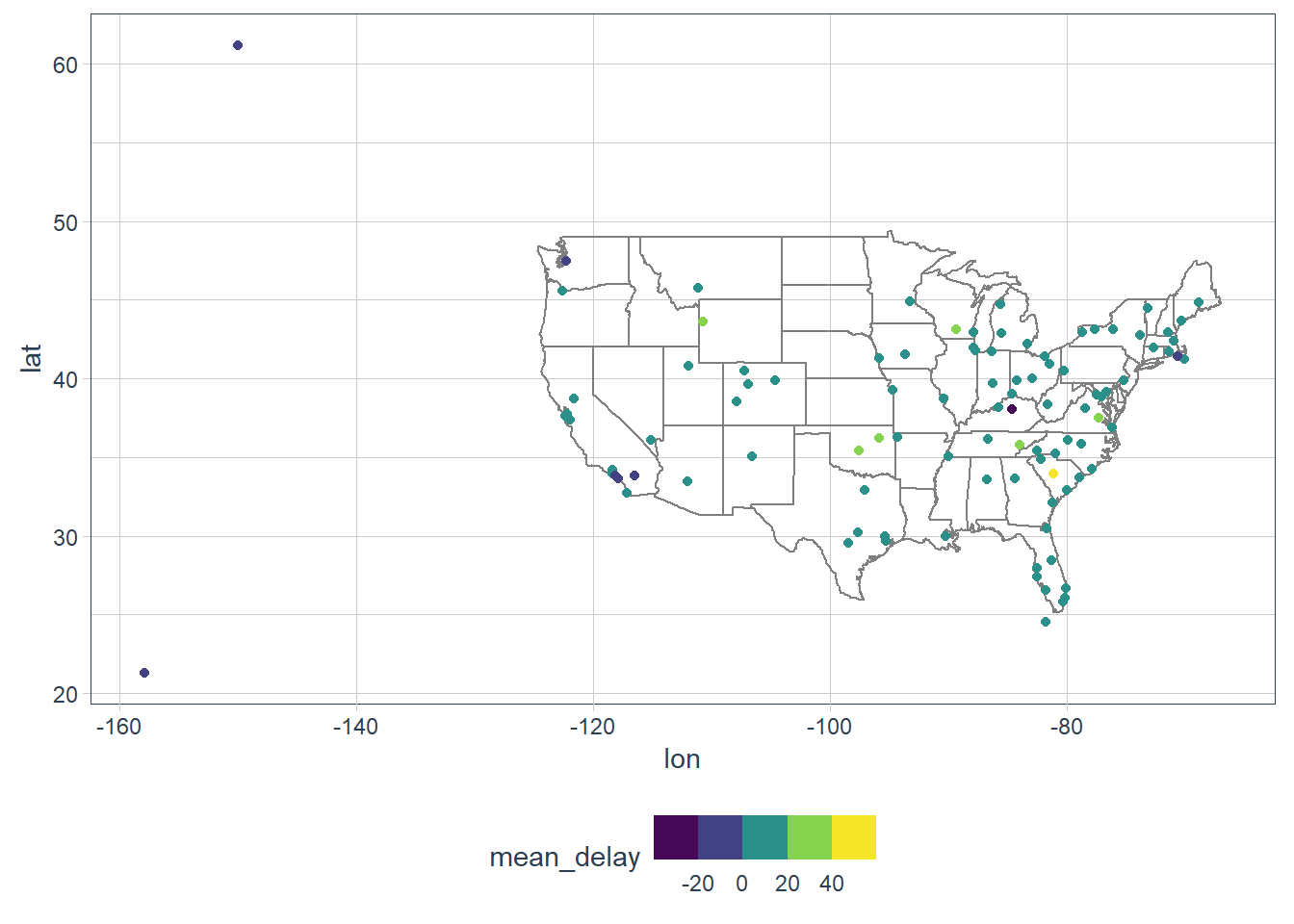
Compute the average delay by destination, then join on the airports data frame so you can show the spatial distribution of delays. Here’s an easy way to draw a map of the United States:

airports %>%
  semi_join(flights, c("faa" = "dest")) %>%
  ggplot(aes(lon, lat)) +
    borders("state") +
    geom_point() +
    coord_quickmap()

(Don’t worry if you don’t understand what semi_join() does — you’ll learn about it next.)

You might want to use the size or colour of the points to display the average delay for each airport.

flights %>% 
  group_by(dest) %>% 
  summarise(mean_delay = mean(arr_delay, na.rm = TRUE)) %>% 
  inner_join(airports, c("dest" = "faa")) %>% 
  ggplot(aes(lon, lat, colour = mean_delay)) +
    borders("state") +
    geom_point() +
    coord_quickmap() +
    scale_colour_viridis_b()

Add the location of the origin and destination (i.e. the lat and lon) to flights.

flights %>% 
  left_join(airports, by = c("origin" = "faa")) %>% 
  left_join(airports, by = c("dest" = "faa")) %>% 
  print(width = Inf)
#> # A tibble: 336,776 x 33
#>     year month   day dep_time sched_dep_time dep_delay arr_time sched_arr_time
#>    <int> <int> <int>    <int>          <int>     <dbl>    <int>          <int>
#>  1  2013     1     1      517            515         2      830            819
#>  2  2013     1     1      533            529         4      850            830
#>  3  2013     1     1      542            540         2      923            850
#>  4  2013     1     1      544            545        -1     1004           1022
#>  5  2013     1     1      554            600        -6      812            837
#>  6  2013     1     1      554            558        -4      740            728
#>  7  2013     1     1      555            600        -5      913            854
#>  8  2013     1     1      557            600        -3      709            723
#>  9  2013     1     1      557            600        -3      838            846
#> 10  2013     1     1      558            600        -2      753            745
#>    arr_delay carrier flight tailnum origin dest  air_time distance  hour minute
#>        <dbl> <chr>    <int> <chr>   <chr>  <chr>    <dbl>    <dbl> <dbl>  <dbl>
#>  1        11 UA        1545 N14228  EWR    IAH        227     1400     5     15
#>  2        20 UA        1714 N24211  LGA    IAH        227     1416     5     29
#>  3        33 AA        1141 N619AA  JFK    MIA        160     1089     5     40
#>  4       -18 B6         725 N804JB  JFK    BQN        183     1576     5     45
#>  5       -25 DL         461 N668DN  LGA    ATL        116      762     6      0
#>  6        12 UA        1696 N39463  EWR    ORD        150      719     5     58
#>  7        19 B6         507 N516JB  EWR    FLL        158     1065     6      0
#>  8       -14 EV        5708 N829AS  LGA    IAD         53      229     6      0
#>  9        -8 B6          79 N593JB  JFK    MCO        140      944     6      0
#> 10         8 AA         301 N3ALAA  LGA    ORD        138      733     6      0
#>    time_hour           name.x              lat.x lon.x alt.x  tz.x dst.x
#>    <dttm>              <chr>               <dbl> <dbl> <dbl> <dbl> <chr>
#>  1 2013-01-01 05:00:00 Newark Liberty Intl  40.7 -74.2    18    -5 A    
#>  2 2013-01-01 05:00:00 La Guardia           40.8 -73.9    22    -5 A    
#>  3 2013-01-01 05:00:00 John F Kennedy Intl  40.6 -73.8    13    -5 A    
#>  4 2013-01-01 05:00:00 John F Kennedy Intl  40.6 -73.8    13    -5 A    
#>  5 2013-01-01 06:00:00 La Guardia           40.8 -73.9    22    -5 A    
#>  6 2013-01-01 05:00:00 Newark Liberty Intl  40.7 -74.2    18    -5 A    
#>  7 2013-01-01 06:00:00 Newark Liberty Intl  40.7 -74.2    18    -5 A    
#>  8 2013-01-01 06:00:00 La Guardia           40.8 -73.9    22    -5 A    
#>  9 2013-01-01 06:00:00 John F Kennedy Intl  40.6 -73.8    13    -5 A    
#> 10 2013-01-01 06:00:00 La Guardia           40.8 -73.9    22    -5 A    
#>    tzone.x          name.y                          lat.y lon.y alt.y  tz.y
#>    <chr>            <chr>                           <dbl> <dbl> <dbl> <dbl>
#>  1 America/New_York George Bush Intercontinental     30.0 -95.3    97    -6
#>  2 America/New_York George Bush Intercontinental     30.0 -95.3    97    -6
#>  3 America/New_York Miami Intl                       25.8 -80.3     8    -5
#>  4 America/New_York <NA>                             NA    NA      NA    NA
#>  5 America/New_York Hartsfield Jackson Atlanta Intl  33.6 -84.4  1026    -5
#>  6 America/New_York Chicago Ohare Intl               42.0 -87.9   668    -6
#>  7 America/New_York Fort Lauderdale Hollywood Intl   26.1 -80.2     9    -5
#>  8 America/New_York Washington Dulles Intl           38.9 -77.5   313    -5
#>  9 America/New_York Orlando Intl                     28.4 -81.3    96    -5
#> 10 America/New_York Chicago Ohare Intl               42.0 -87.9   668    -6
#>    dst.y tzone.y         
#>    <chr> <chr>           
#>  1 A     America/Chicago 
#>  2 A     America/Chicago 
#>  3 A     America/New_York
#>  4 <NA>  <NA>            
#>  5 A     America/New_York
#>  6 A     America/Chicago 
#>  7 A     America/New_York
#>  8 A     America/New_York
#>  9 A     America/New_York
#> 10 A     America/Chicago 
#> # ... with 336,766 more rows

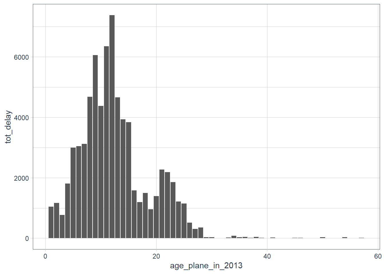
Is there a relationship between the age of a plane and its delays?

Let’s have a look at the total delay, i.e. considering the departure and arrival delays.

(flights_sub <- flights %>% 
   # get subset of fields
   select(year:day, dep_delay, arr_delay, origin, dest,
          tailnum))
#> # A tibble: 336,776 x 8
#>     year month   day dep_delay arr_delay origin dest  tailnum
#>    <int> <int> <int>     <dbl>     <dbl> <chr>  <chr> <chr>  
#>  1  2013     1     1         2        11 EWR    IAH   N14228 
#>  2  2013     1     1         4        20 LGA    IAH   N24211 
#>  3  2013     1     1         2        33 JFK    MIA   N619AA 
#>  4  2013     1     1        -1       -18 JFK    BQN   N804JB 
#>  5  2013     1     1        -6       -25 LGA    ATL   N668DN 
#>  6  2013     1     1        -4        12 EWR    ORD   N39463 
#>  7  2013     1     1        -5        19 EWR    FLL   N516JB 
#>  8  2013     1     1        -3       -14 LGA    IAD   N829AS 
#>  9  2013     1     1        -3        -8 JFK    MCO   N593JB 
#> 10  2013     1     1        -2         8 LGA    ORD   N3ALAA 
#> # ... with 336,766 more rows

flights_sub %>% 
  # join on tailnum
  inner_join(planes, by = ("tailnum" = "tailnum")) %>% 
  # subset data again from the planes tbl
  select(dep_delay, arr_delay, origin, dest,
         tailnum, year.x, year.y,type, manufacturer) %>% 
  # need stats for a plane, so group by tailnum the
  # unique id for a plane
  group_by(tailnum) %>% 
  # add variables to calc age of plane
  # and various delay stats
  mutate(age_plane_in_2013 = year.x - year.y,
         mean_dep_delay = mean(dep_delay, na.rm = TRUE),
         mean_arr_delay = mean(arr_delay, na.rm = TRUE),
         tot_delay = mean_dep_delay + mean_arr_delay) %>% 
  # we only care about planes where delay exists
  # and where we know the planes age
  filter(tot_delay > 0,
         age_plane_in_2013 > 0) %>% 
  select(tailnum, year = year.y, age_plane_in_2013, type, manufacturer,
         mean_dep_delay, mean_arr_delay, tot_delay) %>% 
  ungroup() %>% 
  distinct() %>% 
  ggplot(aes(x = age_plane_in_2013, y = tot_delay)) +
  geom_col()

The planes delay increases as the plane ages, but starts decreasing around age = 12, and drops further past that age. Perhaps the maintenance cycle gets more rigourous as the plane ages? 🤷

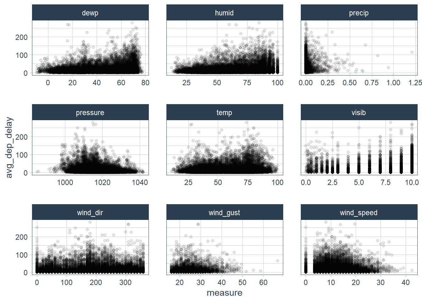
What weather conditions make it more likely to see a delay?


flights %>% 
  select("year", "month", "day", "origin", "hour", "time_hour",
         "dep_delay") %>% 
  inner_join(weather) %>% 
  group_by(origin, year, month, day, hour) %>% 
  mutate(avg_dep_delay = mean(dep_delay, na.rm = TRUE)) %>% 
  ungroup() %>% 
  filter(avg_dep_delay > 0) %>% 
  select("year", "month", "day", "origin", "hour", 
         "avg_dep_delay", "temp":"visib") %>% 
  distinct() %>% 
  arrange(-avg_dep_delay) %>% 
  # slice_head(n = 10) %>% 
  # print(width = Inf) %>% 
  pivot_longer(cols = "temp":"visib",
               names_to = "type",
               values_to = "measure") %>% 
  ggplot(aes(y = avg_dep_delay, x = measure)) +
  geom_point(alpha = 0.1) +
  facet_wrap(~ type, scales = "free_x")

It seems that the higher the dewp and humidity (and to some degree temp) the higher the delay. The visibility in miles also seems to increase the departure delay.

The precipitation seems to decrease the delay which is a bit strange for me, I was under the impression that would lead to longer delays.

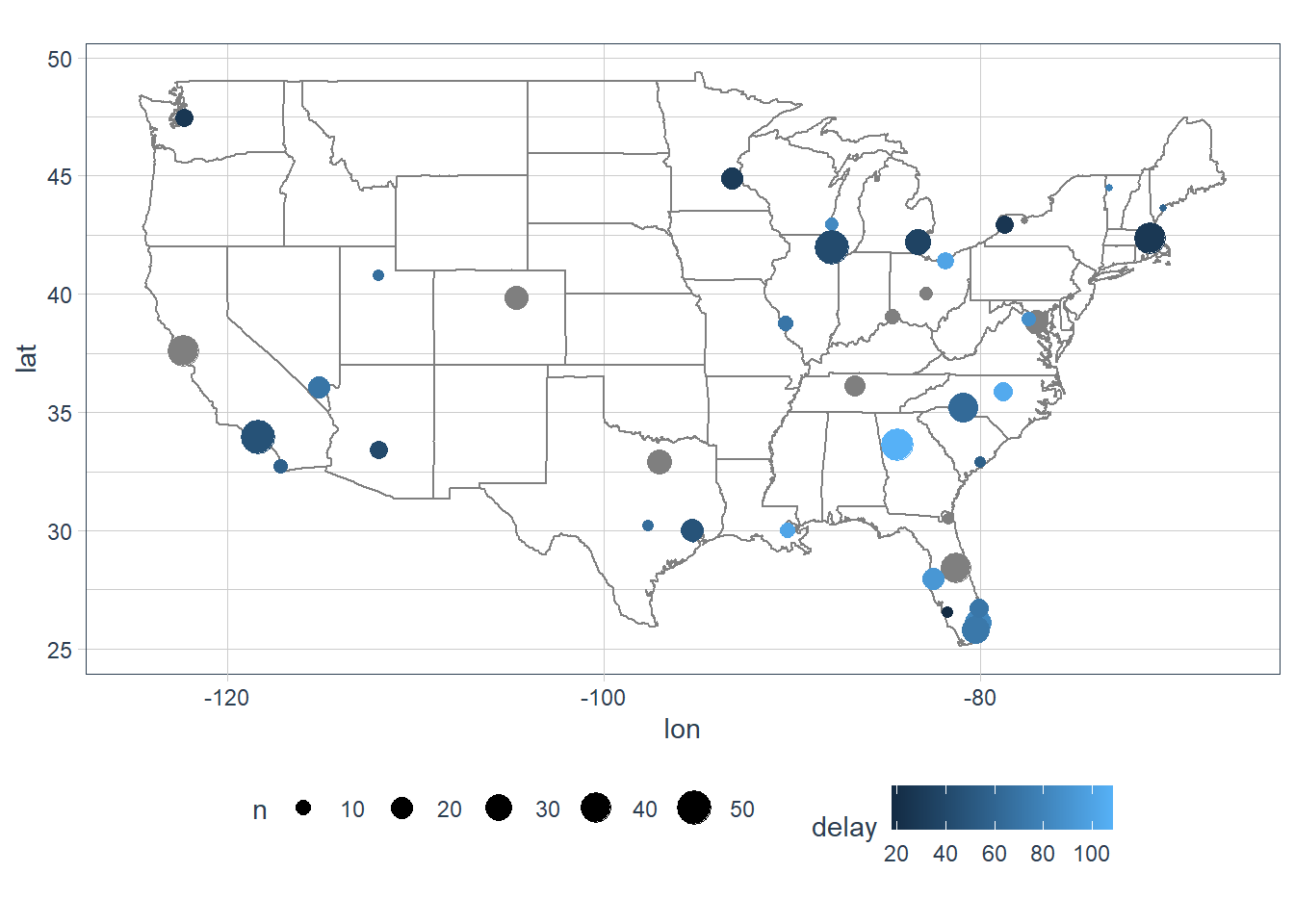
What happened on June 13 2013? Display the spatial pattern of delays, and then use Google to cross-reference with the weather.

worst <- filter(flights, !is.na(dep_time), month == 6, day == 13)
worst %>%
  group_by(dest) %>%
  summarise(delay = mean(arr_delay), n = n()) %>%
  filter(n > 5) %>%
  inner_join(airports, by = c("dest" = "faa")) %>%
  ggplot(aes(lon, lat)) +
    borders("state") +
    geom_point(aes(size = n, colour = delay)) +
    coord_quickmap()

It seems there was intense storms on June 13th, 2013.

Other ways

base::merge() can perform all four types of mutating join:

dplyr	merge
`inner_join(x, y)`	`merge(x, y)`
`left_join(x, y)`	`merge(x, y, all.x = TRUE)`
`right_join(x, y)`	`merge(x, y, all.y = TRUE)`,
`full_join(x, y)`	`merge(x, y, all.x = TRUE, all.y = TRUE)`

Pros for {dplyr}:

Easier to understand what the code is doing,
Translates better to SQL (which is a language by the way, and not an acronym - found out from SQL: Visual QuickStart Guide, by Chris Fehily,
Is faster, and
Does not mess with row order.

SQL translation

dplyr	SQL
`inner_join(x, y, by = "z")`	`SELECT * FROM x INNER JOIN y USING (z)`
`left_join(x, y, by = "z")`	`SELECT * FROM x LEFT OUTER JOIN y USING (z)`
`right_join(x, y, by = "z")`	`SELECT * FROM x RIGHT OUTER JOIN y USING (z)`
`full_join(x, y, by = "z")`	`SELECT * FROM x FULL OUTER JOIN y USING (z)`

Joining different variables between the tables, e.g. inner_join(x, y, by = c("a" = "b")) uses a slightly different syntax in SQL: SELECT * FROM x INNER JOIN y ON x.a = y.b.

Filtering Joins

semi_join(x, y): keeps all observations in x with a corresponding observation in y. Semi-joins are useful for matching filtered summary tables back to the original tbl.

You can think of semi_join(x, y) as observations in x asking each observation in y - “Hey, yoohoo, over there, for the columns we have in common, do you also have the same values in those columns as I do?”
- if yes (doppelgänger found), x observation kept
- if no (no doppelgänger found), x observation dropped
- Keep ONLY the observations of me you can find in y
anti_join(x, y): drops all observations in x that have a match in y. I.e. it keeps the rows that don’t have a match.

You can think of anti_join(x, y) as observations in x asking each observation in y the same question as above, but taking the opposite action!
- if yes (doppelgänger found), x observation dropped [I want to be unique!]
- if no (doppelgänger not found), x observation retained [Yay, I’m the only one]
- Keeps ONLY Unique entries of me

(top_dest <- flights %>%
  count(dest, sort = TRUE) %>%
  head(10))
#> # A tibble: 10 x 2
#>    dest      n
#>    <chr> <int>
#>  1 ORD   17283
#>  2 ATL   17215
#>  3 LAX   16174
#>  4 BOS   15508
#>  5 MCO   14082
#>  6 CLT   14064
#>  7 SFO   13331
#>  8 FLL   12055
#>  9 MIA   11728
#> 10 DCA    9705

Now to find flights that went to one of those destinations you could construct a filter yourself …

flights %>% 
  filter(dest %in% top_dest$dest)
#> # A tibble: 141,145 x 19
#>     year month   day dep_time sched_dep_time dep_delay arr_time sched_arr_time
#>    <int> <int> <int>    <int>          <int>     <dbl>    <int>          <int>
#>  1  2013     1     1      542            540         2      923            850
#>  2  2013     1     1      554            600        -6      812            837
#>  3  2013     1     1      554            558        -4      740            728
#>  4  2013     1     1      555            600        -5      913            854
#>  5  2013     1     1      557            600        -3      838            846
#>  6  2013     1     1      558            600        -2      753            745
#>  7  2013     1     1      558            600        -2      924            917
#>  8  2013     1     1      558            600        -2      923            937
#>  9  2013     1     1      559            559         0      702            706
#> 10  2013     1     1      600            600         0      851            858
#> # ... with 141,135 more rows, and 11 more variables: arr_delay <dbl>,
#> #   carrier <chr>, flight <int>, tailnum <chr>, origin <chr>, dest <chr>,
#> #   air_time <dbl>, distance <dbl>, hour <dbl>, minute <dbl>, time_hour <dttm>

But this gets tricky if you have multiple columns you’re summarising something for.

flights %>% 
  semi_join(top_dest)
#> # A tibble: 141,145 x 19
#>     year month   day dep_time sched_dep_time dep_delay arr_time sched_arr_time
#>    <int> <int> <int>    <int>          <int>     <dbl>    <int>          <int>
#>  1  2013     1     1      542            540         2      923            850
#>  2  2013     1     1      554            600        -6      812            837
#>  3  2013     1     1      554            558        -4      740            728
#>  4  2013     1     1      555            600        -5      913            854
#>  5  2013     1     1      557            600        -3      838            846
#>  6  2013     1     1      558            600        -2      753            745
#>  7  2013     1     1      558            600        -2      924            917
#>  8  2013     1     1      558            600        -2      923            937
#>  9  2013     1     1      559            559         0      702            706
#> 10  2013     1     1      600            600         0      851            858
#> # ... with 141,135 more rows, and 11 more variables: arr_delay <dbl>,
#> #   carrier <chr>, flight <int>, tailnum <chr>, origin <chr>, dest <chr>,
#> #   air_time <dbl>, distance <dbl>, hour <dbl>, minute <dbl>, time_hour <dttm>

How many flights don’t have a match in plane?

flights %>% 
  anti_join(planes, by = "tailnum") %>% 
  count(tailnum, sort = TRUE)
#> # A tibble: 722 x 2
#>    tailnum     n
#>       
#>  1      2512
#>  2 N725MQ    575
#>  3 N722MQ    513
#>  4 N723MQ    507
#>  5 N713MQ    483
#>  6 N735MQ    396
#>  7 N0EGMQ    371
#>  8 N534MQ    364
#>  9 N542MQ    363
#> 10 N531MQ    349
#> # ... with 712 more rows

Exercises

What does it mean for a flight to have a missing tailnum? What do the tail numbers that don’t have a matching record in planes have in common? (Hint: one variable explains ~90% of the problems.)

flights %>% 
  filter(is.na(tailnum),
         is.na(dep_time),
         is.na(dep_delay),
         is.na(arr_time),
         is.na(arr_delay))
#> # A tibble: 2,512 x 19
#>     year month   day dep_time sched_dep_time dep_delay arr_time sched_arr_time
#>    <int> <int> <int>    <int>          <int>     <dbl>    <int>          <int>
#>  1  2013     1     2       NA           1545        NA       NA           1910
#>  2  2013     1     2       NA           1601        NA       NA           1735
#>  3  2013     1     3       NA            857        NA       NA           1209
#>  4  2013     1     3       NA            645        NA       NA            952
#>  5  2013     1     4       NA            845        NA       NA           1015
#>  6  2013     1     4       NA           1830        NA       NA           2044
#>  7  2013     1     5       NA            840        NA       NA           1001
#>  8  2013     1     7       NA            820        NA       NA            958
#>  9  2013     1     8       NA           1645        NA       NA           1838
#> 10  2013     1     9       NA            755        NA       NA           1012
#> # ... with 2,502 more rows, and 11 more variables: arr_delay <dbl>,
#> #   carrier <chr>, flight <int>, tailnum <chr>, origin <chr>, dest <chr>,
#> #   air_time <dbl>, distance <dbl>, hour <dbl>, minute <dbl>, time_hour <dttm>

The flights that were cancelled seem to be the ones with missing tailnum.

What about those that have a tailnum but we don’t have an entry for it in planes?

(missing_planes <- flights %>% 
  anti_join(planes, by = "tailnum") %>% 
  count(tailnum, sort = TRUE))
#> # A tibble: 722 x 2
#>    tailnum     n
#>    <chr>   <int>
#>  1 <NA>     2512
#>  2 N725MQ    575
#>  3 N722MQ    513
#>  4 N723MQ    507
#>  5 N713MQ    483
#>  6 N735MQ    396
#>  7 N0EGMQ    371
#>  8 N534MQ    364
#>  9 N542MQ    363
#> 10 N531MQ    349
#> # ... with 712 more rows

flights %>% 
  filter(!is.na(tailnum)) %>% 
  semi_join(missing_planes, by = "tailnum") %>% 
  select(tailnum, carrier) %>% 
  left_join(airlines, by = "carrier") %>% 
  count(carrier, name, sort = TRUE) 
#> # A tibble: 9 x 3
#>   carrier name                            n
#>   <chr>   <chr>                       <int>
#> 1 MQ      Envoy Air                   25395
#> 2 AA      American Airlines Inc.      22474
#> 3 UA      United Air Lines Inc.        1007
#> 4 B6      JetBlue Airways               830
#> 5 FL      AirTran Airways Corporation   187
#> 6 DL      Delta Air Lines Inc.          110
#> 7 F9      Frontier Airlines Inc.         47
#> 8 US      US Airways Inc.                36
#> 9 WN      Southwest Airlines Co.          8

planes %>% 
   filter(stringr::str_detect(tailnum, "MQ")|
          stringr::str_detect(tailnum, "AA"))
#> # A tibble: 175 x 9
#>    tailnum  year type           manufacturer model engines seats speed engine   
#>    <chr>   <int> <chr>          <chr>        <chr>   <int> <int> <int> <chr>    
#>  1 N201AA   1959 Fixed wing si~ CESSNA       150         1     2    90 Reciproc~
#>  2 N202AA   1980 Fixed wing mu~ CESSNA       421C        2     8    90 Reciproc~
#>  3 N319AA   1985 Fixed wing mu~ BOEING       767-~       2   255    NA Turbo-fan
#>  4 N320AA   1985 Fixed wing mu~ BOEING       767-~       2   255    NA Turbo-fan
#>  5 N323AA   1986 Fixed wing mu~ BOEING       767-~       2   255    NA Turbo-fan
#>  6 N324AA   1986 Fixed wing mu~ BOEING       767-~       2   255    NA Turbo-fan
#>  7 N325AA   1986 Fixed wing mu~ BOEING       767-~       2   255    NA Turbo-fan
#>  8 N327AA   1986 Fixed wing mu~ BOEING       767-~       2   255    NA Turbo-fan
#>  9 N328AA   1986 Fixed wing mu~ BOEING       767-~       2   255    NA Turbo-fan
#> 10 N329AA   1987 Fixed wing mu~ BOEING       767-~       2   255    NA Turbo-fan
#> # ... with 165 more rows

(carrier_missing <- airlines %>% 
  filter(carrier == "MQ" | carrier == "AA"))
#> # A tibble: 2 x 2
#>   carrier name                  
#>   <chr>   <chr>                 
#> 1 AA      American Airlines Inc.
#> 2 MQ      Envoy Air

These seem to be mostly for carriers AA, MQ, which are American Airlines Inc., Envoy Air.

Filter flights to only show flights with planes that have flown at least 100 flights.

(flights_100 <- flights %>% 
   filter(!is.na(tailnum)) %>% 
   select(tailnum) %>% 
   add_count(tailnum) %>% 
   filter(n >= 100)
)
#> # A tibble: 228,390 x 2
#>    tailnum     n
#>    <chr>   <int>
#>  1 N14228    111
#>  2 N24211    130
#>  3 N804JB    219
#>  4 N39463    107
#>  5 N516JB    288
#>  6 N829AS    230
#>  7 N593JB    294
#>  8 N793JB    283
#>  9 N657JB    285
#> 10 N53441    102
#> # ... with 228,380 more rows

flights %>% 
  semi_join(flights_100)
#> # A tibble: 228,390 x 19
#>     year month   day dep_time sched_dep_time dep_delay arr_time sched_arr_time
#>    <int> <int> <int>    <int>          <int>     <dbl>    <int>          <int>
#>  1  2013     1     1      517            515         2      830            819
#>  2  2013     1     1      533            529         4      850            830
#>  3  2013     1     1      544            545        -1     1004           1022
#>  4  2013     1     1      554            558        -4      740            728
#>  5  2013     1     1      555            600        -5      913            854
#>  6  2013     1     1      557            600        -3      709            723
#>  7  2013     1     1      557            600        -3      838            846
#>  8  2013     1     1      558            600        -2      849            851
#>  9  2013     1     1      558            600        -2      853            856
#> 10  2013     1     1      558            600        -2      923            937
#> # ... with 228,380 more rows, and 11 more variables: arr_delay <dbl>,
#> #   carrier <chr>, flight <int>, tailnum <chr>, origin <chr>, dest <chr>,
#> #   air_time <dbl>, distance <dbl>, hour <dbl>, minute <dbl>, time_hour <dttm>

Combine fueleconomy::vehicles and fueleconomy::common to find only the records for the most common models.

fueleconomy::common %>% 
  left_join(fueleconomy::vehicles,
            by = c("make"="make", "model"="model"))
#> # A tibble: 14,531 x 14
#>    make  model     n years    id  year class trans drive   cyl displ fuel    hwy
#>    <chr> <chr> <int> <int> <dbl> <dbl> <chr> <chr> <chr> <dbl> <dbl> <chr> <dbl>
#>  1 Acura Inte~    42    16  1833  1986 Subc~ Auto~ Fron~     4   1.6 Regu~    28
#>  2 Acura Inte~    42    16  1834  1986 Subc~ Manu~ Fron~     4   1.6 Regu~    28
#>  3 Acura Inte~    42    16  3037  1987 Subc~ Auto~ Fron~     4   1.6 Regu~    28
#>  4 Acura Inte~    42    16  3038  1987 Subc~ Manu~ Fron~     4   1.6 Regu~    28
#>  5 Acura Inte~    42    16  4183  1988 Subc~ Auto~ Fron~     4   1.6 Regu~    27
#>  6 Acura Inte~    42    16  4184  1988 Subc~ Manu~ Fron~     4   1.6 Regu~    28
#>  7 Acura Inte~    42    16  5303  1989 Subc~ Auto~ Fron~     4   1.6 Regu~    27
#>  8 Acura Inte~    42    16  5304  1989 Subc~ Manu~ Fron~     4   1.6 Regu~    28
#>  9 Acura Inte~    42    16  6442  1990 Subc~ Auto~ Fron~     4   1.8 Regu~    24
#> 10 Acura Inte~    42    16  6443  1990 Subc~ Manu~ Fron~     4   1.8 Regu~    26
#> # ... with 14,521 more rows, and 1 more variable: cty <dbl>

Find the 48 hours (over the course of the whole year) that have the worst delays. Cross-reference it with the weather data. Can you see any patterns?

I am going to assume that the question just wants the top 48 hours that constitute the worst delays, and not the worst consecutive 48 hour block of time.

flights %>% 
  group_by(year, month, day, hour, origin) %>% 
  summarise(mean_dep_delay = mean(dep_delay, na.rm = TRUE)) %>% 
  # ungroup removes grouping - without this we get weird
  # results! Try it with and without to see diff.
  ungroup() %>% 
  arrange(-mean_dep_delay) %>% 
  slice_head(n = 48) %>% 
  left_join(weather) %>% 
  pivot_longer(cols = temp:visib,
               names_to = "type",
               values_to = "measure") %>% 
  ggplot(aes(y = mean_dep_delay, x = measure )) +
    geom_point(alpha = 0.2) +
    facet_wrap(~ type, scales = "free_x")

If we look at the Defining Key Columns under question 4, we see that these flights with the top delays have humidity in the higher humidity range we saw overall, and same for temperature.

What does anti_join(flights, airports, by = c("dest" = "faa")) tell you? What does anti_join(airports, flights, by = c("faa" = "dest")) tell you?

anti_join(flights, airports, by = c("dest" = "faa"))
#> # A tibble: 7,602 x 19
#>     year month   day dep_time sched_dep_time dep_delay arr_time sched_arr_time
#>    <int> <int> <int>    <int>          <int>     <dbl>    <int>          <int>
#>  1  2013     1     1      544            545        -1     1004           1022
#>  2  2013     1     1      615            615         0     1039           1100
#>  3  2013     1     1      628            630        -2     1137           1140
#>  4  2013     1     1      701            700         1     1123           1154
#>  5  2013     1     1      711            715        -4     1151           1206
#>  6  2013     1     1      820            820         0     1254           1310
#>  7  2013     1     1      820            820         0     1249           1329
#>  8  2013     1     1      840            845        -5     1311           1350
#>  9  2013     1     1      909            810        59     1331           1315
#> 10  2013     1     1      913            918        -5     1346           1416
#> # ... with 7,592 more rows, and 11 more variables: arr_delay <dbl>,
#> #   carrier <chr>, flight <int>, tailnum <chr>, origin <chr>, dest <chr>,
#> #   air_time <dbl>, distance <dbl>, hour <dbl>, minute <dbl>, time_hour <dttm>

anti_join(flights, airports, by = c("dest" = "faa")) %>% 
  distinct(dest)
#> # A tibble: 4 x 1
#>   dest 
#>   <chr>
#> 1 BQN  
#> 2 SJU  
#> 3 STT  
#> 4 PSE

anti_join(airports, flights, by = c("faa" = "dest"))
#> # A tibble: 1,357 x 8
#>    faa   name                       lat    lon   alt    tz dst   tzone          
#>    <chr> <chr>                    <dbl>  <dbl> <dbl> <dbl> <chr> <chr>          
#>  1 04G   Lansdowne Airport         41.1  -80.6  1044    -5 A     America/New_Yo~
#>  2 06A   Moton Field Municipal A~  32.5  -85.7   264    -6 A     America/Chicago
#>  3 06C   Schaumburg Regional       42.0  -88.1   801    -6 A     America/Chicago
#>  4 06N   Randall Airport           41.4  -74.4   523    -5 A     America/New_Yo~
#>  5 09J   Jekyll Island Airport     31.1  -81.4    11    -5 A     America/New_Yo~
#>  6 0A9   Elizabethton Municipal ~  36.4  -82.2  1593    -5 A     America/New_Yo~
#>  7 0G6   Williams County Airport   41.5  -84.5   730    -5 A     America/New_Yo~
#>  8 0G7   Finger Lakes Regional A~  42.9  -76.8   492    -5 A     America/New_Yo~
#>  9 0P2   Shoestring Aviation Air~  39.8  -76.6  1000    -5 U     America/New_Yo~
#> 10 0S9   Jefferson County Intl     48.1 -123.    108    -8 A     America/Los_An~
#> # ... with 1,347 more rows

airports %>% 
  distinct(tz)
#> # A tibble: 7 x 1
#>      tz
#>   <dbl>
#> 1    -5
#> 2    -6
#> 3    -8
#> 4    -7
#> 5    -9
#> 6   -10
#> 7     8

anti_join(flights, airports, by = c("dest" = "faa")) gives us any flights where the destination does not exist in airports.

If you google the airport names you will see that most flight destinations that are not in airports are located in Puerto Rico, or US Virgin Islands. Perhaps these were not in the FAA listing of airports when this data was extracted? Because the wiki pages for these show that the FAA code is the same as we see here.

anti_join(airports, flights, by = c("faa" = "dest")) gives us airports that don’t exist in flights. These will be destinations that are not flown to directing from New York.

You might expect that there’s an implicit relationship between plane and airline, because each plane is flown by a single airline. Confirm or reject this hypothesis using the tools you’ve learned above.

Ok so what would we believe here? I would suspect that a plane belongs to a single airline. But some counters to this view is that surely planes can be bought and sold between carriers. The question would be in that case would the plane change tailnum?

Working on the first assumption what sort of join would help me determine if a plane belongs to one airline?

I would do a left_join(planes, flights, by = "tailnum") and then get the carrier(s) per plane, and join with airlines.
```
flights %>% 
  select(tailnum, carrier) %>% 
  distinct() %>% 
  left_join(airlines, by = "carrier") %>% 
  inner_join(planes, by = "tailnum") %>% 
  count(tailnum, carrier) %>% 
  filter(n > 1)
#> # A tibble: 0 x 3
#> # ... with 3 variables: tailnum <chr>, carrier <chr>, n <int>
```

Tips for joins

Determine the primary key
Check that none of the primary key variables are NULL
Check that foreign keys match primary keys in other tables.
Don’t just rely on counts before and after joins! These can be misleading.

Set operations

intersect(x, y): return only observations in both x and y.
union(x, y): return unique observations in x and y.
setdiff(x, y): return observations in x, but not in y.

df1 <- tribble(
  ~x, ~y,
   1,  1,
   2,  1
)
df2 <- tribble(
  ~x, ~y,
   1,  1,
   1,  2
)

Intersect

dplyr::intersect(df1, df2)
#> # A tibble: 1 x 2
#>       x     y
#>   <dbl> <dbl>
#> 1     1     1

Union

dplyr::union(df1, df2)
#> # A tibble: 3 x 2
#>       x     y
#>   <dbl> <dbl>
#> 1     1     1
#> 2     2     1
#> 3     1     2

Setdiff

setdiff(df1, df2)
#> # A tibble: 1 x 2
#>       x     y
#>   <dbl> <dbl>
#> 1     2     1
setdiff(df2, df1)
#> # A tibble: 1 x 2
#>       x     y
#>   <dbl> <dbl>
#> 1     1     2

sessionInfo()
#> R version 3.6.3 (2020-02-29)
#> Platform: x86_64-w64-mingw32/x64 (64-bit)
#> Running under: Windows 10 x64 (build 18363)
#> 
#> Matrix products: default
#> 
#> locale:
#> [1] LC_COLLATE=English_South Africa.1252  LC_CTYPE=English_South Africa.1252   
#> [3] LC_MONETARY=English_South Africa.1252 LC_NUMERIC=C                         
#> [5] LC_TIME=English_South Africa.1252    
#> 
#> attached base packages:
#> [1] stats     graphics  grDevices utils     datasets  methods   base     
#> 
#> other attached packages:
#>  [1] nycflights13_1.0.1         tidyquant_1.0.0           
#>  [3] quantmod_0.4.17            TTR_0.23-6                
#>  [5] PerformanceAnalytics_2.0.4 xts_0.12-0                
#>  [7] zoo_1.8-7                  magrittr_1.5              
#>  [9] lubridate_1.7.8            emo_0.0.0.9000            
#> [11] flair_0.0.2                forcats_0.5.0             
#> [13] stringr_1.4.0              dplyr_1.0.0               
#> [15] purrr_0.3.4                readr_1.3.1               
#> [17] tidyr_1.1.0                tibble_3.0.3              
#> [19] ggplot2_3.3.0              tidyverse_1.3.0           
#> [21] workflowr_1.6.2           
#> 
#> loaded via a namespace (and not attached):
#>  [1] httr_1.4.2        maps_3.3.0        viridisLite_0.3.0 jsonlite_1.7.0   
#>  [5] modelr_0.1.6      assertthat_0.2.1  cellranger_1.1.0  yaml_2.2.1       
#>  [9] pillar_1.4.6      backports_1.1.6   lattice_0.20-38   glue_1.4.1       
#> [13] quadprog_1.5-8    digest_0.6.25     promises_1.1.0    rvest_0.3.5      
#> [17] colorspace_1.4-1  htmltools_0.5.0   httpuv_1.5.2      fueleconomy_1.0.0
#> [21] pkgconfig_2.0.3   broom_0.5.6       haven_2.2.0       scales_1.1.0     
#> [25] whisker_0.4       later_1.0.0       git2r_0.26.1      farver_2.0.3     
#> [29] generics_0.0.2    ellipsis_0.3.1    DT_0.13           withr_2.2.0      
#> [33] cli_2.0.2         crayon_1.3.4      readxl_1.3.1      Lahman_8.0-0     
#> [37] evaluate_0.14     fs_1.4.1          fansi_0.4.1       nlme_3.1-144     
#> [41] xml2_1.3.2        tools_3.6.3       hms_0.5.3         lifecycle_0.2.0  
#> [45] munsell_0.5.0     reprex_0.3.0      compiler_3.6.3    rlang_0.4.7      
#> [49] grid_3.6.3        rstudioapi_0.11   htmlwidgets_1.5.1 crosstalk_1.1.0.1
#> [53] labeling_0.3      rmarkdown_2.4     gtable_0.3.0      DBI_1.1.0        
#> [57] curl_4.3          R6_2.4.1          knitr_1.28        utf8_1.1.4       
#> [61] rprojroot_1.3-2   Quandl_2.10.0     stringi_1.4.6     Rcpp_1.0.4.6     
#> [65] vctrs_0.3.2       dbplyr_1.4.3      tidyselect_1.1.0  xfun_0.13

Chapter 10 - Relational Data with {dplyr}

Vebash Naidoo

26/10/2020

Relational Data

Main types of joins

Main types of joins

Dataset

Exercises

Keys

Keys

Exercises

Mutating joins

Mutating joins

Inner Join

Outer Joins

Left Join

Right Join

Full Join

Duplicate Keys

Defining Key Columns

Defining Key Columns

Exercises

Other ways

Filtering Joins

Filtering Joins

Exercises

Tips for joins

Set operations

Set operations

Intersect

Union

Setdiff