Compara métodos de campo y dron (paper SUDOE)
ajpelu
2022-04-18
Last updated: 2022-04-19
Checks: 7 0
Knit directory:
veg_alcontar/
This reproducible R Markdown analysis was created with workflowr (version 1.7.0). The Checks tab describes the reproducibility checks that were applied when the results were created. The Past versions tab lists the development history.
Great! Since the R Markdown file has been committed to the Git repository, you know the exact version of the code that produced these results.
Great job! The global environment was empty. Objects defined in the global environment can affect the analysis in your R Markdown file in unknown ways. For reproduciblity it’s best to always run the code in an empty environment.
The command set.seed(20211007) was run prior to running the code in the R Markdown file.
Setting a seed ensures that any results that rely on randomness, e.g.
subsampling or permutations, are reproducible.
Great job! Recording the operating system, R version, and package versions is critical for reproducibility.
Nice! There were no cached chunks for this analysis, so you can be confident that you successfully produced the results during this run.
Great job! Using relative paths to the files within your workflowr project makes it easier to run your code on other machines.
Great! You are using Git for version control. Tracking code development and connecting the code version to the results is critical for reproducibility.
The results in this page were generated with repository version 586d4b9. See the Past versions tab to see a history of the changes made to the R Markdown and HTML files.
Note that you need to be careful to ensure that all relevant files for the
analysis have been committed to Git prior to generating the results (you can
use wflow_publish or wflow_git_commit). workflowr only
checks the R Markdown file, but you know if there are other scripts or data
files that it depends on. Below is the status of the Git repository when the
results were generated:
Ignored files:
    Ignored:    .Rhistory
    Ignored:    .Rproj.user/

Untracked files:
    Untracked:  data/Cobertura_fitovolumen_corregido_parcela.xlsx

Unstaged changes:
    Modified:   analysis/_site.yml
    Modified:   output/paper_SUDOE/compara_cobertura.jpg
Note that any generated files, e.g. HTML, png, CSS, etc., are not included in this status report because it is ok for generated content to have uncommitted changes.
These are the previous versions of the repository in which changes were made
to the R Markdown (analysis/compara_methods_SUDOE.Rmd) and HTML (docs/compara_methods_SUDOE.html)
files. If you’ve configured a remote Git repository (see
?wflow_git_remote), click on the hyperlinks in the table below to
view the files as they were in that past version.
| File | Version | Author | Date | Message |
|---|---|---|---|---|
| Rmd | 586d4b9 | ajpelu | 2022-04-19 | add new analysis organized |
1 Objetivo 1. Carga de combustible: cobertura y fitovolumen
1.1 Cobetura
Vamos a realizar la comparación seleccionando para cada parcela (n=12) un valor de cobertura de quadrats (quadrats medio).
1.1.1 Summary values
| metodo | mean | sd | se | cv | median | min | max | n |
|---|---|---|---|---|---|---|---|---|
| line_intercept | 27.19 | 6.49 | 1.87 | 23.86 | 29.67 | 11.95 | 34.0 | 12 |
| point_quadrat | 55.50 | 7.62 | 2.20 | 13.73 | 56.00 | 41.00 | 64.0 | 12 |
| quadrat medio | 29.92 | 5.35 | 1.54 | 17.88 | 30.81 | 21.25 | 37.5 | 12 |
1.1.2 Comparación de métodos
- ANOVA Kruskal Wallis
| statistic | p.value | parameter | method | mi_variable |
|---|---|---|---|---|
| 23.84398 | 6.6e-06 | 2 | Kruskal-Wallis rank sum test | cobertura |
Los resultados de la ANOVA no paramétrica (Kruskal-Wallis) indican que existen diferencias significativas para la cobertura (%) entre los diferentes métodos de campo empleados (\(\chi^2\) = 23.84; p<0.0001) (Tabla 1.2).
Posteriormente, evaluamos si existen diferencias entre cada uno de los métodos (post hoc) y observamos que existen diferencias significativas entre el point quadrat y los otros métodos (line intercept y quadrat medio) (Tabla 1.3, Figura 1.1). Asimismo, no observamos diferencias entre la cobertura estimada según el line intercept y el quadrat medio.
| H0 | statistic | p.value |
|---|---|---|
| line_intercept = point_quadrat | 4.53 | <0.001 |
| line_intercept = quadrat medio | 0.70 | >0.999 |
| point_quadrat = quadrat medio | 3.84 | <0.001 |
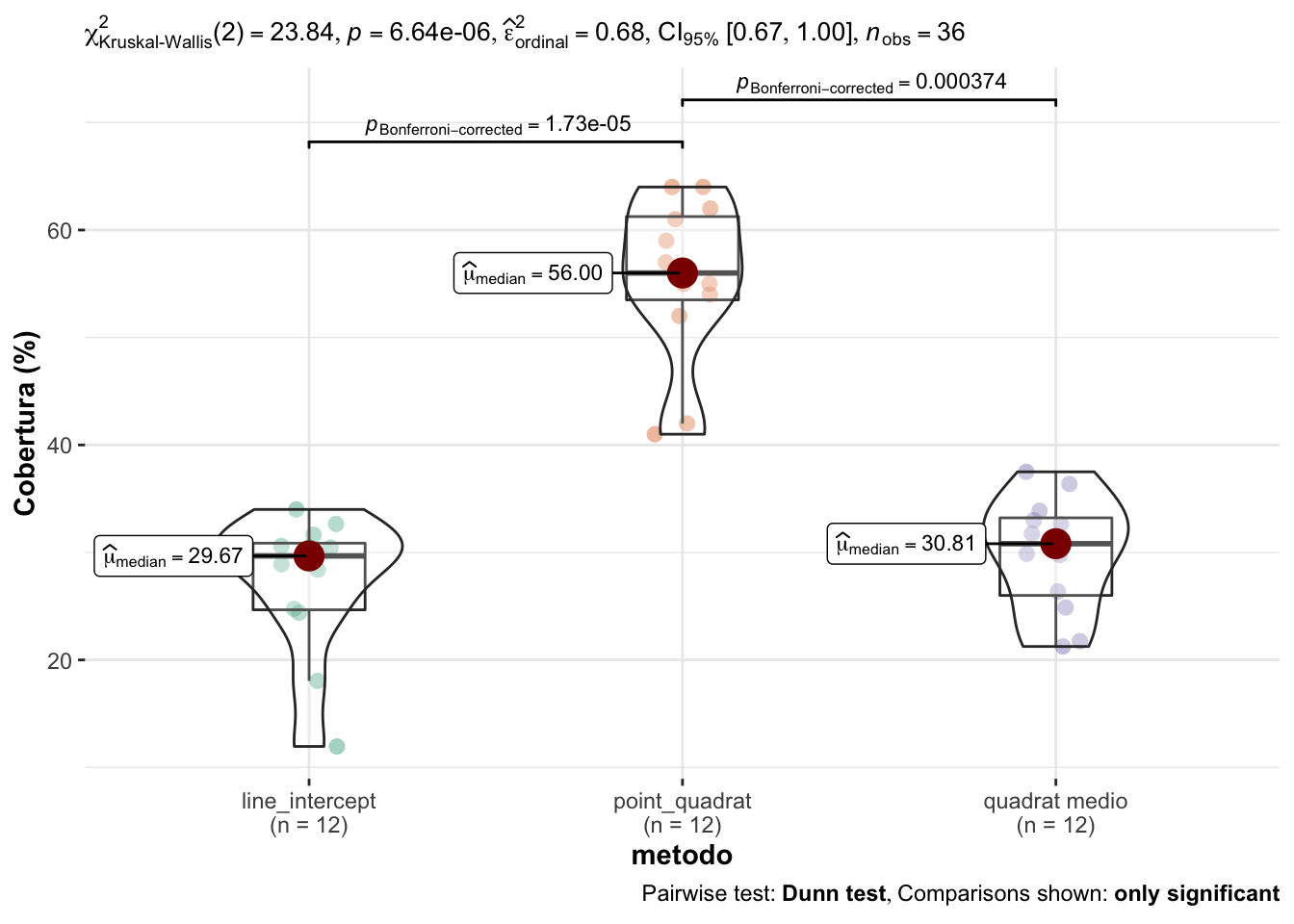
Figure 1.1: Comparación de los valores de cobertura entre los diferentes métodos de campo.
1.1.3 Correlación
El siguiente paso es evaluar la correlación que existe entre los métodos de campo para la cobertura.
Tal y como observamos en la Figura 1.2, existe una correlación significativa del line intercept con el point quadrat (\(R^2=\) 0.63), aunque lejos del ajuste perfecto (línea negra en Figura 1.2). El método point quadrat sobreestima los valores de cobertura con respecto al método de line intercept. Así, el rango de cobertura estimado por el LI varía entre 11.95-34 %, mientras que la estimación por PQ varía entre 41-64% (Tabla 1.1).
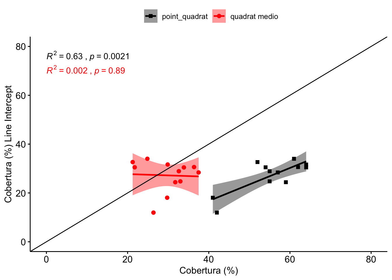
Figure 1.2: Correlación entre los valores de cobertura estimados por Line Intercept y los otros métodos de campo: Point Quadrat y Quadrat medio.
1.2 Fitovolumen
- En este caso solo compararemos los métodos de Line Intercept y Quadrat medio
1.2.1 Summary values
| metodo | mean | sd | se | cv | median | min | max | n |
|---|---|---|---|---|---|---|---|---|
| line_intercept | 531.04 | 274.90 | 79.36 | 51.77 | 543.13 | 84.27 | 1016.86 | 12 |
| quadrat medio | 778.57 | 275.23 | 79.45 | 35.35 | 699.70 | 324.04 | 1296.47 | 12 |
1.2.2 Comparación de métodos
Hemos comprobado Normalidad (W = 0.97; p=0.6350); y homocedasticidad (Bartlett’s K-squared = 0; p=0.9969) y se puede aplicar un método paramétrico, en este caso, la t-student de comparación de medias. Observamos que existen diferencias (Figura 1.3):
The Welch Two Sample t-test testing the difference of value by metodo (mean in group line_intercept = 531.04, mean in group quadrat medio = 778.57) suggests that the effect is negative, statistically significant, and large (difference = -247.53, 95% CI [-480.42, -14.64], t(22.00) = -2.20, p = 0.038; Cohen's d = -0.94, 95% CI [-1.81, -0.05])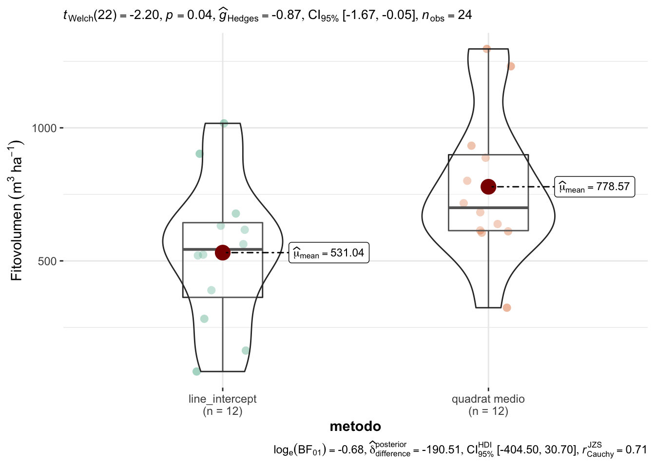
Figure 1.3: Comparación de los valores de fitovolumen entre Line Intercept y Quadrat medio.
1.2.3 Correlación
No existe una buena correlación entre los valores de fitovolumen estimados con line intercept y los estimados con quadrat medio (Figura 1.4). Este último método sobreestima el fitovolumen registrado por el LI (ver Tabla 1.4).
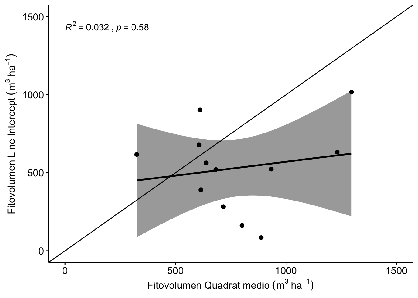
Figure 1.4: Correlación entre los valores de fitovolumen estimados por Line Intercept y Quadrat medio.
R version 4.0.2 (2020-06-22)
Platform: x86_64-apple-darwin17.0 (64-bit)
Running under: macOS Catalina 10.15.3

Matrix products: default
BLAS:   /Library/Frameworks/R.framework/Versions/4.0/Resources/lib/libRblas.dylib
LAPACK: /Library/Frameworks/R.framework/Versions/4.0/Resources/lib/libRlapack.dylib

locale:
[1] en_US.UTF-8/en_US.UTF-8/en_US.UTF-8/C/en_US.UTF-8/en_US.UTF-8

attached base packages:
[1] stats     graphics  grDevices utils     datasets  methods   base

other attached packages:
 [1] multcompView_0.1-8        statsExpressions_1.3.1
 [3] ggsignif_0.6.3            pairwiseComparisons_3.1.3
 [5] ggtext_0.1.1              PMCMRplus_1.9.3
 [7] PMCMR_4.3                 statmod_1.4.36
 [9] tweedie_2.3.3             report_0.5.1
[11] kableExtra_1.3.1          cvequality_0.2.0
[13] performance_0.8.0         ggdist_3.0.1
[15] Metrics_0.1.4             ggstatsplot_0.9.1
[17] colorspace_2.0-2          ggpubr_0.4.0
[19] ggforce_0.3.2             ggdark_0.2.1
[21] janitor_2.1.0             here_1.0.1
[23] forcats_0.5.1             stringr_1.4.0
[25] dplyr_1.0.6               purrr_0.3.4
[27] readr_1.4.0               tidyr_1.1.3
[29] tibble_3.1.2              ggplot2_3.3.5
[31] tidyverse_1.3.1           workflowr_1.7.0

loaded via a namespace (and not attached):
  [1] utf8_1.1.4             tidyselect_1.1.1       grid_4.0.2
  [4] gmp_0.6-2              munsell_0.5.0          codetools_0.2-18
  [7] effectsize_0.6.0.1     withr_2.4.1            highr_0.8
 [10] knitr_1.31             rstudioapi_0.13        ipmisc_5.0.2
 [13] labeling_0.4.2         emmeans_1.5.4          git2r_0.28.0
 [16] polyclip_1.10-0        farver_2.1.0           datawizard_0.4.0
 [19] rprojroot_2.0.2        coda_0.19-4            vctrs_0.3.8
 [22] generics_0.1.0         TH.data_1.0-10         xfun_0.23
 [25] BWStest_0.2.2          R6_2.5.1               BayesFactor_0.9.12-4.3
 [28] cachem_1.0.4           reshape_0.8.8          assertthat_0.2.1
 [31] promises_1.2.0.1       scales_1.1.1.9000      multcomp_1.4-16
 [34] gtable_0.3.0           processx_3.5.1         sandwich_3.0-0
 [37] rlang_0.4.12           MatrixModels_0.4-1     zeallot_0.1.0
 [40] splines_4.0.2          rstatix_0.6.0          broom_0.7.9
 [43] prismatic_1.0.0        yaml_2.2.1             abind_1.4-5
 [46] modelr_0.1.8           backports_1.2.1        httpuv_1.5.5
 [49] gridtext_0.1.4         tools_4.0.2            bookdown_0.21.6
 [52] ellipsis_0.3.2         jquerylib_0.1.3        WRS2_1.1-3
 [55] Rcpp_1.0.7             plyr_1.8.6             ps_1.5.0
 [58] pbapply_1.4-3          correlation_0.8.0      zoo_1.8-8
 [61] haven_2.3.1            ggrepel_0.9.1          fs_1.5.0
 [64] magrittr_2.0.1         data.table_1.14.0      openxlsx_4.2.3
 [67] reprex_2.0.0           mvtnorm_1.1-1          whisker_0.4
 [70] hms_1.0.0              patchwork_1.1.1        evaluate_0.14
 [73] xtable_1.8-4           rio_0.5.16             readxl_1.3.1
 [76] compiler_4.0.2         crayon_1.4.1           htmltools_0.5.2
 [79] mgcv_1.8-33            mc2d_0.1-18            later_1.1.0.1
 [82] lubridate_1.7.10       DBI_1.1.1              SuppDists_1.1-9.5
 [85] kSamples_1.2-9         tweenr_1.0.1           dbplyr_2.1.1
 [88] MASS_7.3-53            boot_1.3-26            Matrix_1.3-2
 [91] car_3.0-10             cli_2.5.0              parallel_4.0.2
 [94] insight_0.17.0         pkgconfig_2.0.3        getPass_0.2-2
 [97] foreign_0.8-81         xml2_1.3.2             paletteer_1.3.0
[100] bslib_0.2.4            webshot_0.5.2          estimability_1.3
[103] rvest_1.0.0            snakecase_0.11.0       distributional_0.3.0
[106] callr_3.7.0            digest_0.6.27          parameters_0.17.0
[109] rmarkdown_2.8          cellranger_1.1.0       curl_4.3
[112] gtools_3.8.2           lifecycle_1.0.1        nlme_3.1-152
[115] jsonlite_1.7.2         carData_3.0-4          viridisLite_0.4.0
[118] fansi_0.4.2            pillar_1.6.1           lattice_0.20-41
[121] fastmap_1.1.0          httr_1.4.2             survival_3.2-7
[124] glue_1.4.2             bayestestR_0.11.5      zip_2.1.1
[127] stringi_1.7.4          sass_0.3.1             rematch2_2.1.2
[130] memoise_2.0.0          Rmpfr_0.8-2