Temporal evolution of veg. parameters by rangos (Spanish)
Antonio J. Pérez-Luque
2022-01-17
Last updated: 2022-01-18
Checks: 7 0
Knit directory: veg_alcontar/
This reproducible R Markdown analysis was created with workflowr (version 1.7.0). The Checks tab describes the reproducibility checks that were applied when the results were created. The Past versions tab lists the development history.
Great! Since the R Markdown file has been committed to the Git repository, you know the exact version of the code that produced these results.
Great job! The global environment was empty. Objects defined in the global environment can affect the analysis in your R Markdown file in unknown ways. For reproduciblity it’s best to always run the code in an empty environment.
The command set.seed(20211007) was run prior to running the code in the R Markdown file. Setting a seed ensures that any results that rely on randomness, e.g. subsampling or permutations, are reproducible.
Great job! Recording the operating system, R version, and package versions is critical for reproducibility.
Nice! There were no cached chunks for this analysis, so you can be confident that you successfully produced the results during this run.
Great job! Using relative paths to the files within your workflowr project makes it easier to run your code on other machines.
Great! You are using Git for version control. Tracking code development and connecting the code version to the results is critical for reproducibility.
The results in this page were generated with repository version fd05b4a. See the Past versions tab to see a history of the changes made to the R Markdown and HTML files.
Note that you need to be careful to ensure that all relevant files for the analysis have been committed to Git prior to generating the results (you can use wflow_publish or wflow_git_commit). workflowr only checks the R Markdown file, but you know if there are other scripts or data files that it depends on. Below is the status of the Git repository when the results were generated:
Ignored files:
    Ignored:    .Rhistory
    Ignored:    .Rproj.user/

Untracked files:
    Untracked:  analysis/ndvi_pastoreo.Rmd
    Untracked:  analysis/tasa_consumo.Rmd
    Untracked:  analysis/temporal_all_EPs.Rmd
    Untracked:  data/Datos_para correlaciones_Antonio.xlsx
    Untracked:  data/Resultados_todos los partners.xlsx
    Untracked:  data/Tablas_horas_pastoreo_EP_V3.xlsx
    Untracked:  data/s2ndvi.csv
    Untracked:  data/tablas_horas_pastoreo.xlsx

Unstaged changes:
    Modified:   analysis/temporal_analysis.Rmd
    Modified:   output/congreso_forestal/cobertura.jpg
    Modified:   output/congreso_forestal/fitovol.jpg
    Modified:   output/congreso_forestal/riqueza.jpg
    Modified:   output/congreso_forestal/shannon.jpg
    Modified:   output/congreso_forestal/tabla_anovas.xls
    Modified:   output/congreso_forestal/tabla_modelos_resumen.xls
    Modified:   output/congreso_forestal/tabla_modelos_smooth.xls
    Deleted:    output/congreso_forestal/~$tabla_congreso_all_metrics.xlsx
Note that any generated files, e.g. HTML, png, CSS, etc., are not included in this status report because it is ok for generated content to have uncommitted changes.
These are the previous versions of the repository in which changes were made to the R Markdown (analysis/temporal_analysis_rangos.Rmd) and HTML (docs/temporal_analysis_rangos.html) files. If you’ve configured a remote Git repository (see ?wflow_git_remote), click on the hyperlinks in the table below to view the files as they were in that past version.
| File | Version | Author | Date | Message |
|---|---|---|---|---|
| Rmd | fd05b4a | ajpelu | 2022-01-18 | improve tables and figures |
| Rmd | e845f96 | ajpelu | 2022-01-17 | update analysis |
| html | e845f96 | ajpelu | 2022-01-17 | update analysis |
Introdución y Objetivos
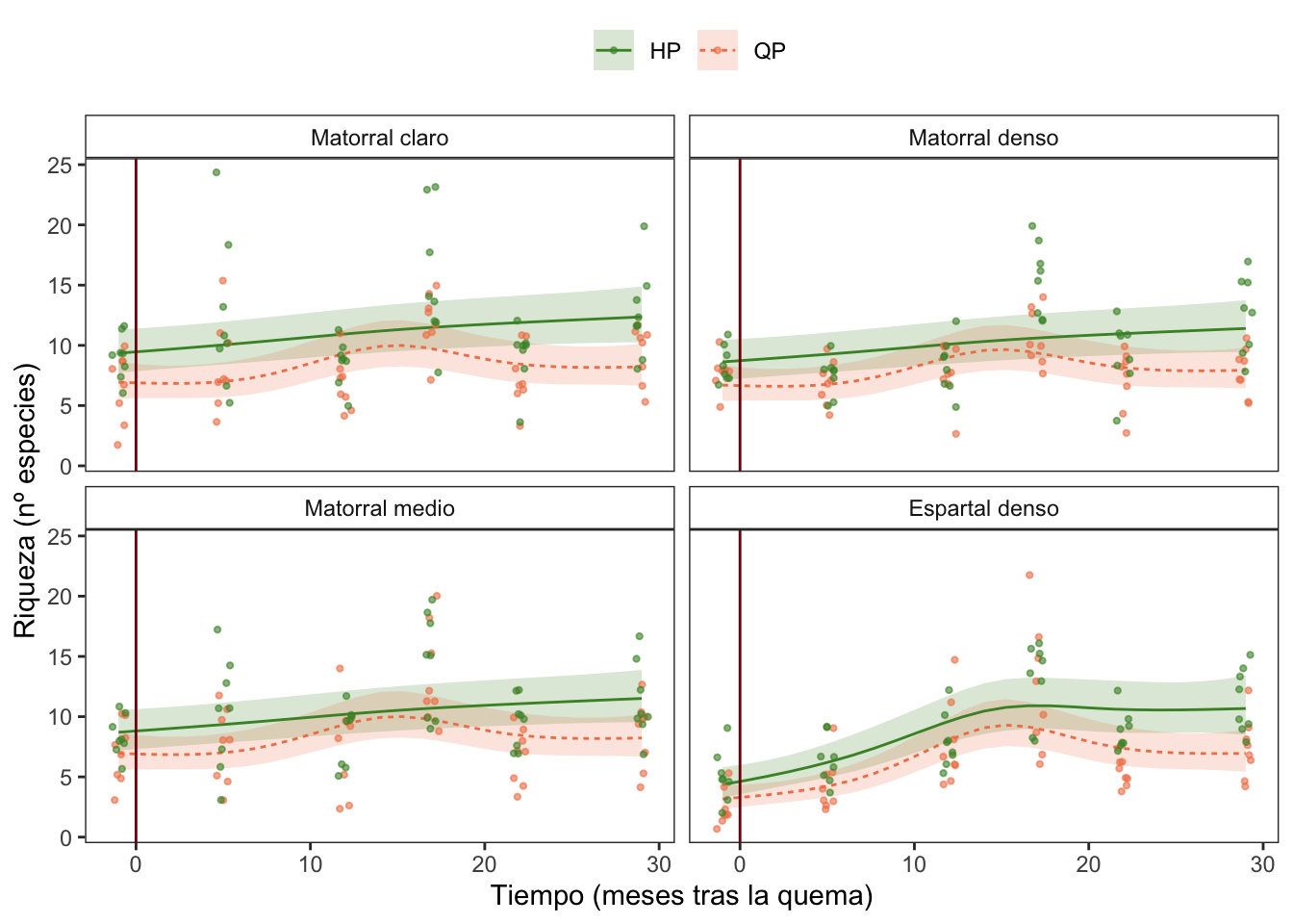
Analizar la evolución de los parámetros de vegetación a lo largo del tiempo, entre dos tratamientos: Herbivorísmo pírico (HP) y Quemas Prescritas (QP), considerando los diferentes rangos
Usamos solamente datos de la quema de Otoño
Diseño:
- tratamiento: HP y QP
- rangos
- 6 fechas de muestreo
- 32 plots por tratamiento
     rango
treat Matorral claro Matorral denso Matorral medio Espartal denso
   HP             48             48             48             48
   QP             48             48             48             48
Análisis estadístico
- Se utilizaron Modelos Mixtos Aditivos Generalizados (GAMM) para evaluar los efectos del tratamiento (Quemas Prescritos vs. Herbivorismo Pírico) sobre la evolución de la cobertura vegetal, el fitovolumen y los índices de diversidad (Shannon, Riqueza).
Riqueza
Modelo
f <- as.formula(
  riq ~
    s(meses, by = interaction(treat, rango), k = 5, bs = "cs") +
    s(meses, by = treat, k = 5, bs = "cs") +
    s(meses, by = rango, k = 5, bs = "cs") +
    treat * rango
)

fi <- as.formula(
  riq ~
    s(meses, by = interaction(treat, rango), k = 5, bs = "cs") +
    treat * rango
)

fni <- as.formula(
  riq ~
    s(meses, by = treat, k = 5, bs = "cs") +
    s(meses, by = rango, k = 5, bs = "cs") +
    treat * rango
)


mfull <- gamm(f,
          random = list(quadrat = ~1),
          data = veg,
          family = poisson,
          method = "ML")
Maximum number of PQL iterations: 20 mi <- gamm(fi,
random = list(quadrat = ~1),
data = veg,
family = poisson,
method = "ML")
Maximum number of PQL iterations: 20 mni <- gamm(fni,
random = list(quadrat = ~1),
data = veg,
family = poisson,
method = "ML")
Maximum number of PQL iterations: 20 - Seleccionamos los suavizados, y elegimos el modelo con menor AIC
| model | df | AIC |
|---|---|---|
| mni | 15 | 319.8728 |
| mfull | 23 | 334.4627 |
| mi | 17 | 336.0228 |
# Distribution of Model Family

Predicted Distribution of Residuals

 Distribution Probability
       normal         66%
      tweedie         34%

Predicted Distribution of Response

               Distribution Probability
              beta-binomial         59%
          negative binomial         12%
 neg. binomial (zero-infl.)          9%
Model validation
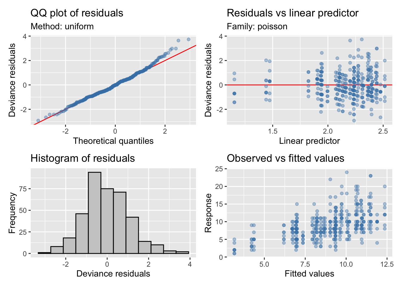
| Version | Author | Date |
|---|---|---|
| e845f96 | ajpelu | 2022-01-17 |
| A. parametric coefficients | Estimate | Std. Error | t-value | p-value |
| (Intercept) | 2.3946 | 0.0854 | 28.0294 | < 0.0001 |
| treatQP | -0.2895 | 0.1234 | -2.3454 | 0.0195 |
| rangoMatorral denso | -0.0806 | 0.1214 | -0.6637 | 0.5073 |
| rangoMatorral medio | -0.0714 | 0.1214 | -0.5883 | 0.5567 |
| rangoEspartal denso | -0.2813 | 0.1236 | -2.2766 | 0.0234 |
| treatQP:rangoMatorral denso | 0.0457 | 0.1752 | 0.2607 | 0.7945 |
| treatQP:rangoMatorral medio | 0.0729 | 0.1749 | 0.4169 | 0.6770 |
| treatQP:rangoEspartal denso | -0.0214 | 0.1781 | -0.1201 | 0.9045 |
| B. smooth terms | edf | Ref.df | F-value | p-value |
| s(meses):treatHP | 1.6005 | 4.0000 | 4.1012 | 0.0001 |
| s(meses):treatQP | 3.4564 | 4.0000 | 6.4054 | < 0.0001 |
| s(meses):rangoMatorral claro | 0.0000 | 4.0000 | 0.0000 | 0.9918 |
| s(meses):rangoMatorral denso | 0.0000 | 4.0000 | 0.0000 | 0.5012 |
| s(meses):rangoMatorral medio | 0.0000 | 4.0000 | 0.0000 | 0.7363 |
| s(meses):rangoEspartal denso | 2.7565 | 4.0000 | 7.5048 | < 0.0001 |
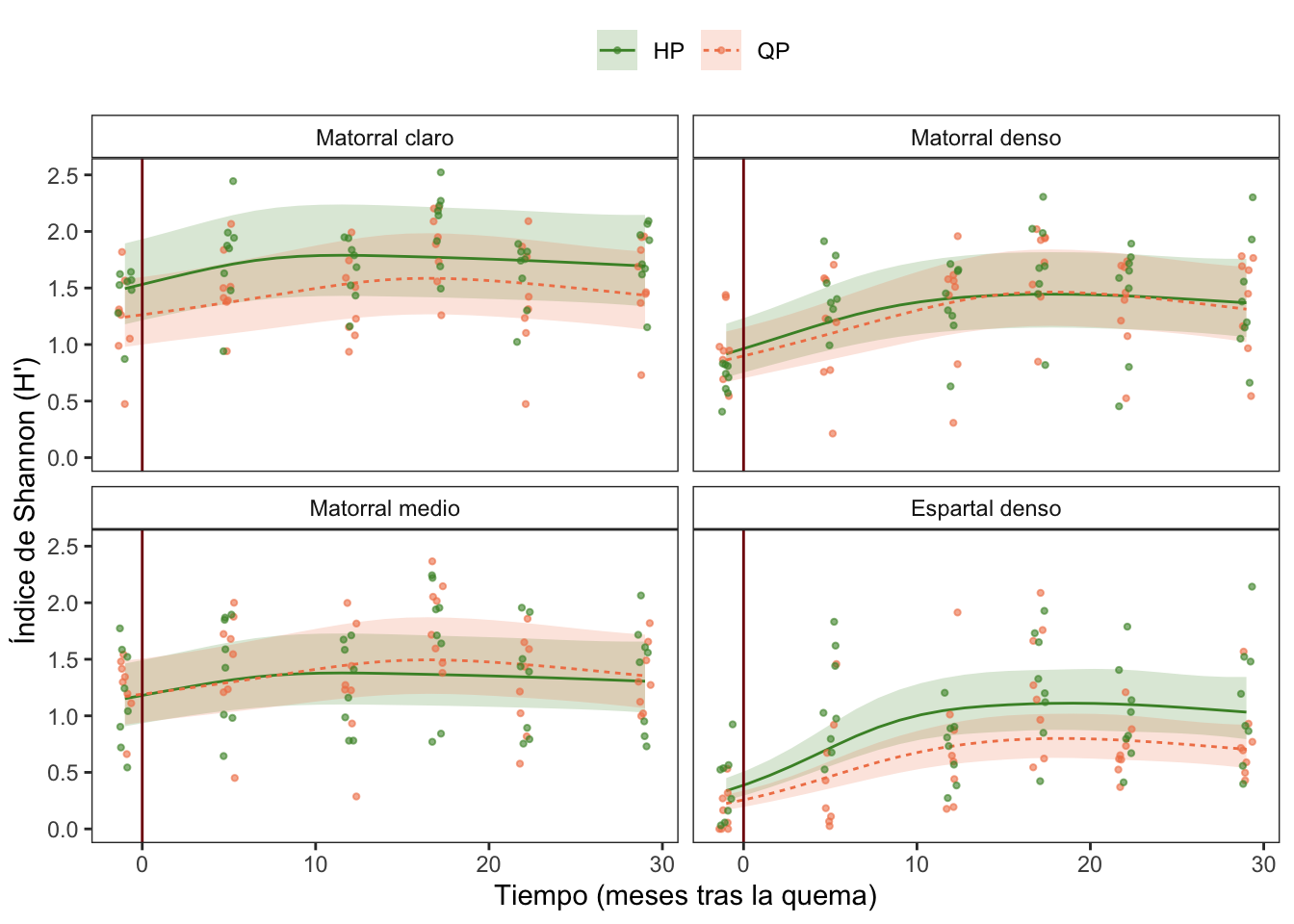
Diversidad
Modelo
f <- as.formula(
  shan ~
    s(meses, by = interaction(treat, rango), k = 5, bs = "cs") +
    s(meses, by = treat, k = 5, bs = "cs") +
    s(meses, by = rango, k = 5, bs = "cs") +
    treat * rango
)

fi <- as.formula(
  shan ~
    s(meses, by = interaction(treat, rango), k = 5, bs = "cs") +
    treat * rango
)

fni <- as.formula(
  shan ~
    s(meses, by = treat, k = 5, bs = "cs") +
    s(meses, by = rango, k = 5, bs = "cs") +
    treat * rango
)


mfull <- gamm(f,
          random = list(quadrat = ~1),
          data = veg,
          family = tw,
          method = "ML")
Maximum number of PQL iterations: 20 mi <- gamm(fi,
random = list(quadrat = ~1),
data = veg,
family = tw,
method = "ML")
Maximum number of PQL iterations: 20 mni <- gamm(fni,
random = list(quadrat = ~1),
data = veg,
family = tw,
method = "ML")
Maximum number of PQL iterations: 20 - Seleccionamos los suavizados, y elegimos el modelo con menor AIC
| model | df | AIC |
|---|---|---|
| mni | 16 | 312.3255 |
| mi | 18 | 326.0420 |
| mfull | 24 | 329.8889 |
# Distribution of Model Family

Predicted Distribution of Residuals

 Distribution Probability
       normal         62%
      tweedie         19%
         beta         12%

Predicted Distribution of Response

 Distribution Probability
      tweedie         47%
      weibull         25%
         beta         12%
Model validation
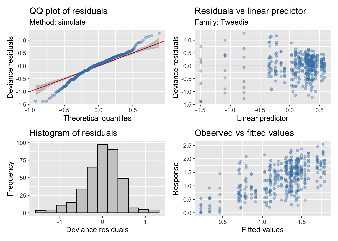
| Version | Author | Date |
|---|---|---|
| e845f96 | ajpelu | 2022-01-17 |
| A. parametric coefficients | Estimate | Std. Error | t-value | p-value |
| (Intercept) | 0.5287 | 0.1110 | 4.7639 | < 0.0001 |
| treatQP | -0.1583 | 0.1573 | -1.0059 | 0.3151 |
| rangoMatorral denso | -0.2817 | 0.1576 | -1.7872 | 0.0747 |
| rangoMatorral medio | -0.2605 | 0.1576 | -1.6529 | 0.0992 |
| rangoEspartal denso | -0.7181 | 0.1590 | -4.5166 | < 0.0001 |
| treatQP:rangoMatorral denso | 0.1236 | 0.2233 | 0.5535 | 0.5803 |
| treatQP:rangoMatorral medio | 0.2017 | 0.2231 | 0.9042 | 0.3665 |
| treatQP:rangoEspartal denso | -0.2180 | 0.2258 | -0.9652 | 0.3351 |
| B. smooth terms | edf | Ref.df | F-value | p-value |
| s(meses):treatHP | 2.3165 | 4.0000 | 2.1678 | 0.0131 |
| s(meses):treatQP | 2.2922 | 4.0000 | 3.6264 | 0.0006 |
| s(meses):rangoMatorral claro | 0.0000 | 4.0000 | 0.0000 | 0.5747 |
| s(meses):rangoMatorral denso | 1.8420 | 4.0000 | 2.6999 | 0.0022 |
| s(meses):rangoMatorral medio | 0.0000 | 4.0000 | 0.0000 | 0.5277 |
| s(meses):rangoEspartal denso | 3.0818 | 4.0000 | 20.0725 | < 0.0001 |
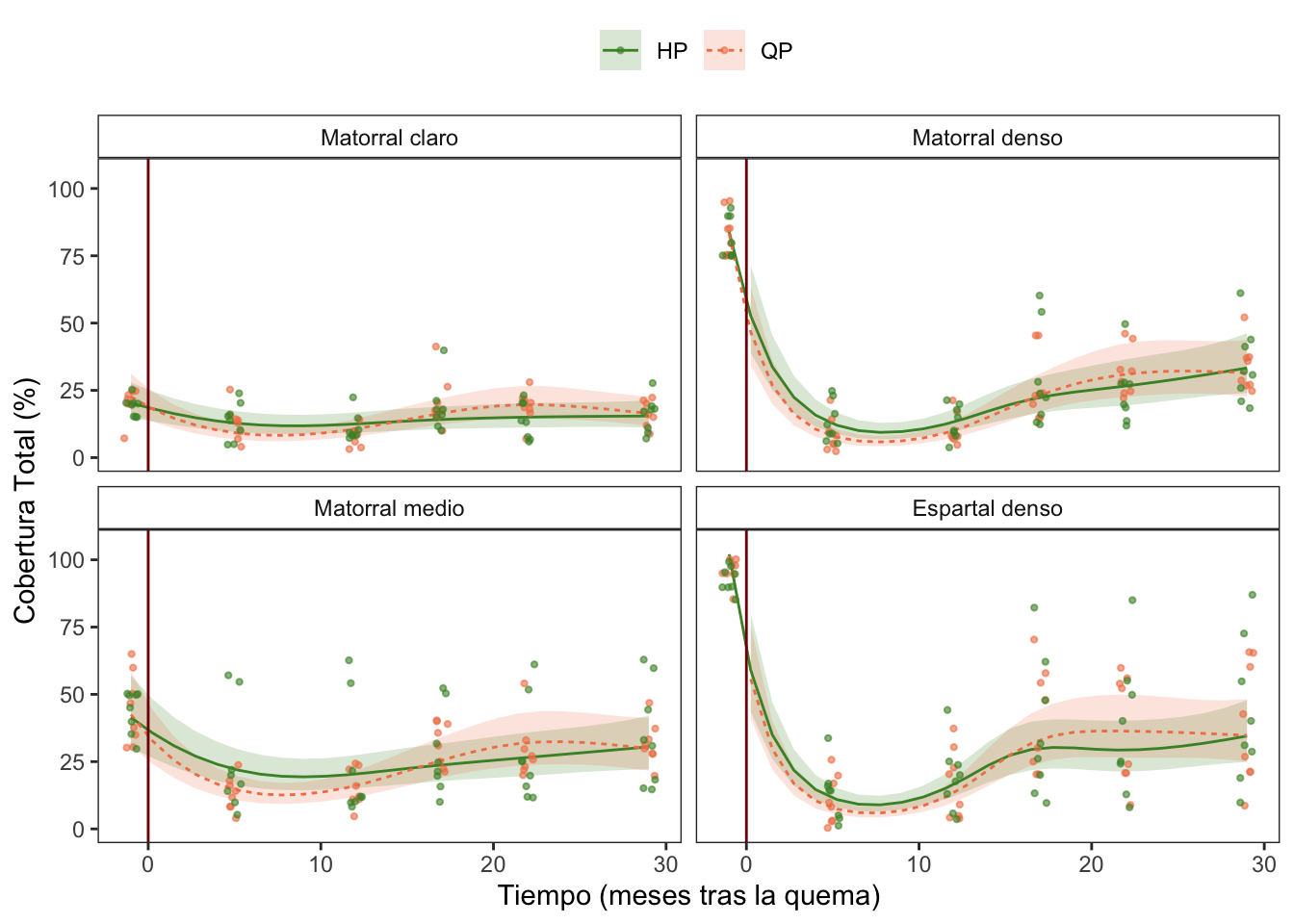
Cobertura
Modelo
f <- as.formula(
  cob ~
    s(meses, by = interaction(treat, rango), k = 5, bs = "cs") +
    s(meses, by = treat, k = 5, bs = "cs") +
    s(meses, by = rango, k = 5, bs = "cs") +
    treat * rango
)

fi <- as.formula(
  cob ~
    s(meses, by = interaction(treat, rango), k = 5, bs = "cs") +
    treat * rango
)

fni <- as.formula(
  cob ~
    s(meses, by = treat, k = 5, bs = "cs") +
    s(meses, by = rango, k = 5, bs = "cs") +
    treat * rango
)


mfull <- gamm(f,
          random = list(quadrat = ~1),
          data = veg,
          family = nb,
          method = "ML")
Maximum number of PQL iterations: 20 mi <- gamm(fi,
random = list(quadrat = ~1),
data = veg,
family = nb,
method = "ML")
Maximum number of PQL iterations: 20 mni <- gamm(fni,
random = list(quadrat = ~1),
data = veg,
family = nb,
method = "ML")
Maximum number of PQL iterations: 20 - Seleccionamos los suavizados, y elegimos el modelo con menor AIC
| model | df | AIC |
|---|---|---|
| mni | 16 | 553.3551 |
| mfull | 24 | 569.3556 |
| mi | 18 | 604.5710 |
# Distribution of Model Family

Predicted Distribution of Residuals

 Distribution Probability
       normal         69%
      tweedie         28%
         beta          3%

Predicted Distribution of Response

               Distribution Probability
 neg. binomial (zero-infl.)         91%
              beta-binomial          9%
Model validation
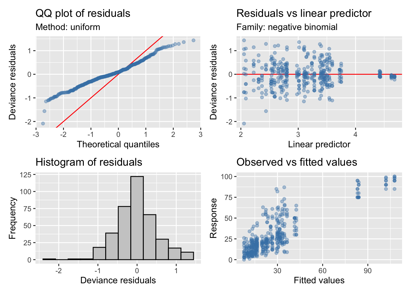
| Version | Author | Date |
|---|---|---|
| e845f96 | ajpelu | 2022-01-17 |
| A. parametric coefficients | Estimate | Std. Error | t-value | p-value |
| (Intercept) | 2.6987 | 0.1387 | 19.4558 | < 0.0001 |
| treatQP | 0.0166 | 0.1962 | 0.0846 | 0.9326 |
| rangoMatorral denso | 0.5418 | 0.1960 | 2.7644 | 0.0060 |
| rangoMatorral medio | 0.5852 | 0.1960 | 2.9861 | 0.0030 |
| rangoEspartal denso | 0.6656 | 0.1960 | 3.3959 | 0.0008 |
| treatQP:rangoMatorral denso | -0.1166 | 0.2773 | -0.4206 | 0.6743 |
| treatQP:rangoMatorral medio | -0.0813 | 0.2772 | -0.2934 | 0.7694 |
| treatQP:rangoEspartal denso | -0.0529 | 0.2772 | -0.1909 | 0.8487 |
| B. smooth terms | edf | Ref.df | F-value | p-value |
| s(meses):treatHP | 3.2434 | 4.0000 | 5.4764 | < 0.0001 |
| s(meses):treatQP | 3.7914 | 4.0000 | 21.8033 | < 0.0001 |
| s(meses):rangoMatorral claro | 0.0000 | 4.0000 | 0.0000 | 0.1724 |
| s(meses):rangoMatorral denso | 3.8000 | 4.0000 | 25.9436 | < 0.0001 |
| s(meses):rangoMatorral medio | 1.9142 | 4.0000 | 1.1067 | 0.0882 |
| s(meses):rangoEspartal denso | 3.8968 | 4.0000 | 33.2093 | < 0.0001 |
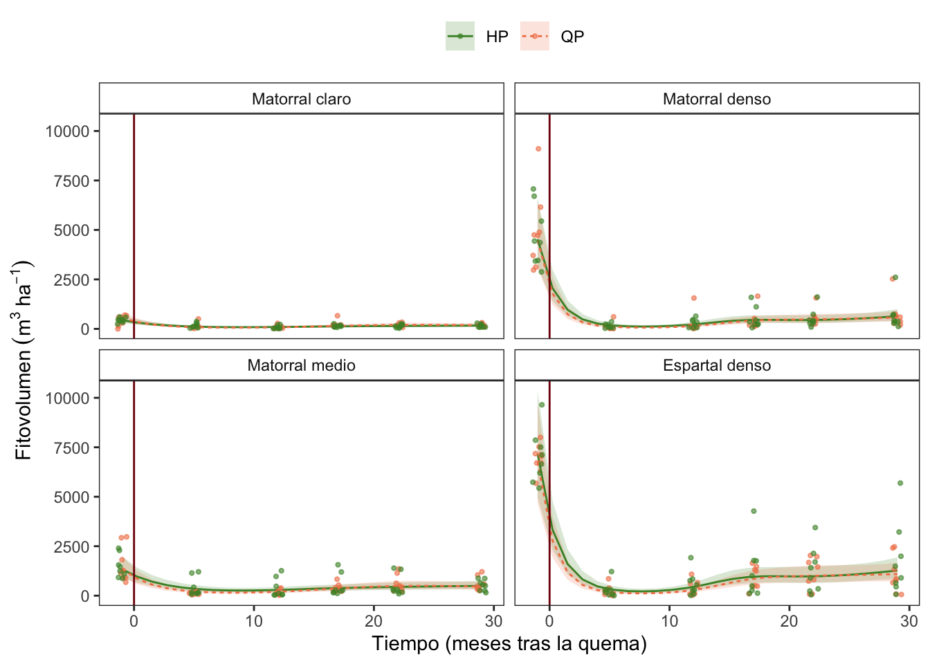
Fitovolumen
Modelo
f <- as.formula(
  fitovol ~
    s(meses, by = interaction(treat, rango), k = 5, bs = "cs") +
    s(meses, by = treat, k = 5, bs = "cs") +
    s(meses, by = rango, k = 5, bs = "cs") +
    treat * rango
)

fi <- as.formula(
  fitovol ~
    s(meses, by = interaction(treat, rango), k = 5, bs = "cs") +
    treat * rango
)

fni <- as.formula(
  fitovol ~
    s(meses, by = treat, k = 5, bs = "cs") +
    s(meses, by = rango, k = 5, bs = "cs") +
    treat * rango
)


mfull <- gamm(f,
          random = list(quadrat = ~1),
          data = veg,
          family = tw,
          method = "ML")
Maximum number of PQL iterations: 20 mi <- gamm(fi,
random = list(quadrat = ~1),
data = veg,
family = tw,
method = "ML")
Maximum number of PQL iterations: 20 mni <- gamm(fni,
random = list(quadrat = ~1),
data = veg,
family = tw,
method = "ML")
Maximum number of PQL iterations: 20 - Seleccionamos los suavizados, y elegimos el modelo con menor AIC
| model | df | AIC |
|---|---|---|
| mni | 16 | 903.7188 |
| mfull | 24 | 919.8060 |
| mi | 18 | 958.6921 |
# Distribution of Model Family

Predicted Distribution of Residuals

 Distribution Probability
       normal         53%
      tweedie         47%

Predicted Distribution of Response

 Distribution Probability
    lognormal         31%
      tweedie         22%
            F         16%
Model validation
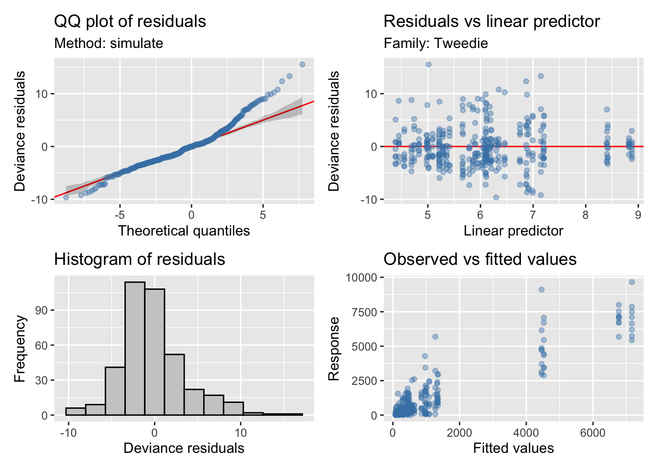
| Version | Author | Date |
|---|---|---|
| e845f96 | ajpelu | 2022-01-17 |
| A. parametric coefficients | Estimate | Std. Error | t-value | p-value |
| (Intercept) | 5.0453 | 0.1969 | 25.6224 | < 0.0001 |
| treatQP | 0.0576 | 0.2773 | 0.2076 | 0.8357 |
| rangoMatorral denso | 1.2420 | 0.2682 | 4.6310 | < 0.0001 |
| rangoMatorral medio | 1.1151 | 0.2685 | 4.1532 | < 0.0001 |
| rangoEspartal denso | 1.8986 | 0.2648 | 7.1699 | < 0.0001 |
| treatQP:rangoMatorral denso | -0.2339 | 0.3765 | -0.6212 | 0.5348 |
| treatQP:rangoMatorral medio | -0.2065 | 0.3794 | -0.5443 | 0.5866 |
| treatQP:rangoEspartal denso | -0.2753 | 0.3724 | -0.7391 | 0.4603 |
| B. smooth terms | edf | Ref.df | F-value | p-value |
| s(meses):treatHP | 3.5747 | 4.0000 | 29.5108 | < 0.0001 |
| s(meses):treatQP | 3.7773 | 4.0000 | 42.6866 | < 0.0001 |
| s(meses):rangoMatorral claro | 0.0000 | 4.0000 | 0.0000 | 0.7831 |
| s(meses):rangoMatorral denso | 3.7580 | 4.0000 | 22.1492 | < 0.0001 |
| s(meses):rangoMatorral medio | 0.0000 | 4.0000 | 0.0000 | 0.7361 |
| s(meses):rangoEspartal denso | 3.7961 | 4.0000 | 19.4941 | < 0.0001 |
Overall
- Smooth terms
Variable term edf ref.df F p Richness s(meses):treatHP 1.601 4 4.10 < 0.001 Richness s(meses):treatQP 3.456 4 6.40 < 0.001 Richness s(meses):rangoMatorral claro 0.000 4 0.00 0.992 Richness s(meses):rangoMatorral denso 0.000 4 0.00 0.501 Richness s(meses):rangoMatorral medio 0.000 4 0.00 0.736 Richness s(meses):rangoEspartal denso 2.756 4 7.50 < 0.001 Shannon s(meses):treatHP 2.317 4 2.17 0.013 Shannon s(meses):treatQP 2.292 4 3.63 0.001 Shannon s(meses):rangoMatorral claro 0.000 4 0.00 0.575 Shannon s(meses):rangoMatorral denso 1.842 4 2.70 0.002 Shannon s(meses):rangoMatorral medio 0.000 4 0.00 0.528 Shannon s(meses):rangoEspartal denso 3.082 4 20.07 < 0.001 Cobertura total s(meses):treatHP 3.243 4 5.48 < 0.001 Cobertura total s(meses):treatQP 3.791 4 21.80 < 0.001 Cobertura total s(meses):rangoMatorral claro 0.000 4 0.00 0.172 Cobertura total s(meses):rangoMatorral denso 3.800 4 25.94 < 0.001 Cobertura total s(meses):rangoMatorral medio 1.914 4 1.11 0.088 Cobertura total s(meses):rangoEspartal denso 3.897 4 33.21 < 0.001 Fitovolumen s(meses):treatHP 3.575 4 29.51 < 0.001 Fitovolumen s(meses):treatQP 3.777 4 42.69 < 0.001 Fitovolumen s(meses):rangoMatorral claro 0.000 4 0.00 0.783 Fitovolumen s(meses):rangoMatorral denso 3.758 4 22.15 < 0.001 Fitovolumen s(meses):rangoMatorral medio 0.000 4 0.00 0.736 Fitovolumen s(meses):rangoEspartal denso 3.796 4 19.49 < 0.001 - Parametrics terms
| Variable | param. terms | df | F | p.value |
|---|---|---|---|---|
| Richness | treat | 1 | 5.501 | 0.02 |
| Richness | rango | 3 | 1.880 | 0.132 |
| Richness | treat:rango | 3 | 0.116 | 0.951 |
| Shannon | treat | 1 | 1.012 | 0.315 |
| Shannon | rango | 3 | 6.971 | < 0.001 |
| Shannon | treat:rango | 3 | 1.302 | 0.273 |
| Cobertura total | treat | 1 | 0.007 | 0.933 |
| Cobertura total | rango | 3 | 4.781 | 0.003 |
| Cobertura total | treat:rango | 3 | 0.063 | 0.979 |
| Fitovolumen | treat | 1 | 0.043 | 0.836 |
| Fitovolumen | rango | 3 | 17.379 | < 0.001 |
| Fitovolumen | treat:rango | 3 | 0.207 | 0.892 |
| Variable | R2 | AIC | Model distribution |
|---|---|---|---|
| Richness | 0.262 | 319.87 | Poisson |
| Shannon | 0.384 | 312.33 | Tweedie |
| Cobertura total | 0.698 | 553.36 | Negative Binomial |
| Fitovol | 0.839 | 903.72 | Tweedie |
R version 4.0.2 (2020-06-22)
Platform: x86_64-apple-darwin17.0 (64-bit)
Running under: macOS Catalina 10.15.3

Matrix products: default
BLAS:   /Library/Frameworks/R.framework/Versions/4.0/Resources/lib/libRblas.dylib
LAPACK: /Library/Frameworks/R.framework/Versions/4.0/Resources/lib/libRlapack.dylib

locale:
[1] en_US.UTF-8/en_US.UTF-8/en_US.UTF-8/C/en_US.UTF-8/en_US.UTF-8

attached base packages:
[1] stats     graphics  grDevices utils     datasets  methods   base

other attached packages:
 [1] emmeans_1.5.4     plotrix_3.8-1     gtsummary_1.4.2   patchwork_1.1.1
 [5] performance_0.8.0 broom_0.7.9       tidymv_3.2.1      kableExtra_1.3.1
 [9] itsadug_2.4       plotfunctions_1.4 gratia_0.6.0      mgcv_1.8-33
[13] nlme_3.1-152      janitor_2.1.0     here_1.0.1        forcats_0.5.1
[17] stringr_1.4.0     dplyr_1.0.6       purrr_0.3.4       readr_1.4.0
[21] tidyr_1.1.3       tibble_3.1.2      ggplot2_3.3.5     tidyverse_1.3.1
[25] workflowr_1.7.0

loaded via a namespace (and not attached):
 [1] TH.data_1.0-10      colorspace_2.0-2    ellipsis_0.3.2
 [4] rprojroot_2.0.2     estimability_1.3    snakecase_0.11.0
 [7] fs_1.5.0            rstudioapi_0.13     farver_2.1.0
[10] fansi_0.4.2         mvtnorm_1.1-1       lubridate_1.7.10
[13] xml2_1.3.2          codetools_0.2-18    splines_4.0.2
[16] knitr_1.31          jsonlite_1.7.2      gt_0.3.0
[19] dbplyr_2.1.1        compiler_4.0.2      httr_1.4.2
[22] backports_1.2.1     assertthat_0.2.1    Matrix_1.3-2
[25] fastmap_1.1.0       cli_2.5.0           later_1.1.0.1
[28] htmltools_0.5.2     tools_4.0.2         coda_0.19-4
[31] gtable_0.3.0        glue_1.4.2          Rcpp_1.0.7
[34] cellranger_1.1.0    jquerylib_0.1.3     vctrs_0.3.8
[37] broom.helpers_1.4.0 insight_0.14.4      xfun_0.23
[40] ps_1.5.0            rvest_1.0.0         lifecycle_1.0.1
[43] getPass_0.2-2       MASS_7.3-53         zoo_1.8-8
[46] scales_1.1.1.9000   ragg_1.1.1          hms_1.0.0
[49] promises_1.2.0.1    sandwich_3.0-0      yaml_2.2.1
[52] mvnfast_0.2.7       sass_0.3.1          stringi_1.7.4
[55] highr_0.8           bayestestR_0.9.0    randomForest_4.6-14
[58] systemfonts_1.0.0   rlang_0.4.12        pkgconfig_2.0.3
[61] evaluate_0.14       lattice_0.20-41     labeling_0.4.2
[64] processx_3.5.1      tidyselect_1.1.1    magrittr_2.0.1
[67] R6_2.5.1            generics_0.1.0      multcomp_1.4-16
[70] DBI_1.1.1           pillar_1.6.1        haven_2.3.1
[73] whisker_0.4         withr_2.4.1         survival_3.2-7
[76] modelr_0.1.8        crayon_1.4.1        utf8_1.1.4
[79] rmarkdown_2.8       grid_4.0.2          readxl_1.3.1
[82] callr_3.7.0         git2r_0.28.0        reprex_2.0.0
[85] digest_0.6.27       webshot_0.5.2       xtable_1.8-4
[88] httpuv_1.5.5        textshaping_0.3.2   munsell_0.5.0
[91] tweedie_2.3.3       viridisLite_0.4.0   bslib_0.2.4