Exercise-1-GWAS

workflowr

• Summary
• Checks
• Past versions

Last updated: 2024-01-20

Checks: 6 1

Knit directory: QBS-statsgen/

This reproducible R Markdown analysis was created with workflowr (version 1.6.2). The Checks tab describes the reproducibility checks that were applied when the results were created. The Past versions tab lists the development history.

---

R Markdown file: uncommitted changes

The R Markdown file has unstaged changes. To know which version of the R Markdown file created these results, you’ll want to first commit it to the Git repo. If you’re still working on the analysis, you can ignore this warning. When you’re finished, you can run wflow_publish to commit the R Markdown file and build the HTML.

Environment: empty

Great job! The global environment was empty. Objects defined in the global environment can affect the analysis in your R Markdown file in unknown ways. For reproduciblity it’s best to always run the code in an empty environment.

Seed: set.seed(20231230)

The command set.seed(20231230) was run prior to running the code in the R Markdown file. Setting a seed ensures that any results that rely on randomness, e.g. subsampling or permutations, are reproducible.

Session information: recorded

Great job! Recording the operating system, R version, and package versions is critical for reproducibility.

Cache: none

Nice! There were no cached chunks for this analysis, so you can be confident that you successfully produced the results during this run.

File paths: relative

Great job! Using relative paths to the files within your workflowr project makes it easier to run your code on other machines.

Repository version: 1cb2d1e

Great! You are using Git for version control. Tracking code development and connecting the code version to the results is critical for reproducibility.

The results in this page were generated with repository version 1cb2d1e. See the Past versions tab to see a history of the changes made to the R Markdown and HTML files.

Note that you need to be careful to ensure that all relevant files for the analysis have been committed to Git prior to generating the results (you can use wflow_publish or wflow_git_commit). workflowr only checks the R Markdown file, but you know if there are other scripts or data files that it depends on. Below is the status of the Git repository when the results were generated:

Ignored files:
    Ignored:    .Rproj.user/B81CBE6F/bibliography-index/
    Ignored:    .Rproj.user/B81CBE6F/ctx/
    Ignored:    .Rproj.user/B81CBE6F/pcs/
    Ignored:    .Rproj.user/B81CBE6F/presentation/
    Ignored:    .Rproj.user/B81CBE6F/profiles-cache/
    Ignored:    .Rproj.user/B81CBE6F/sources/per/
    Ignored:    .Rproj.user/B81CBE6F/tutorial/
    Ignored:    .Rproj.user/shared/notebooks/1C2AC29C-e1-gwas-power/
    Ignored:    .Rproj.user/shared/notebooks/1EB0B2DC-e1-gwas/1/B81CBE6Fe0e7218a/
    Ignored:    .Rproj.user/shared/notebooks/1EB0B2DC-e1-gwas/1/s/ce0r78nx8keuu/
    Ignored:    .Rproj.user/shared/notebooks/1EB0B2DC-e1-gwas/1/s/csetup_chunk/
    Ignored:    .Rproj.user/shared/notebooks/1EB0B2DC-e1-gwas/1/s/czxn6jf8lsykc/
    Ignored:    output/

Untracked files:
    Untracked:  temp.csv

Unstaged changes:
    Modified:   .Rproj.user/B81CBE6F/persistent-state
    Modified:   .Rproj.user/B81CBE6F/sources/prop/3814FE49
    Modified:   .Rproj.user/B81CBE6F/sources/prop/4C8B7780
    Modified:   .Rproj.user/B81CBE6F/sources/prop/BBFFB970
    Modified:   .Rproj.user/B81CBE6F/sources/prop/INDEX
    Modified:   .Rproj.user/B81CBE6F/sources/s-e0e7218a/34A40D3B
    Modified:   .Rproj.user/B81CBE6F/sources/s-e0e7218a/6C1FFABC
    Modified:   .Rproj.user/B81CBE6F/sources/s-e0e7218a/6C1FFABC-contents
    Modified:   .Rproj.user/shared/notebooks/1EB0B2DC-e1-gwas/1/s/chunks.json
    Modified:   .Rproj.user/shared/notebooks/paths
    Modified:   analysis/e1-gwas-power.Rmd
    Modified:   analysis/e1-gwas.Rmd

Note that any generated files, e.g. HTML, png, CSS, etc., are not included in this status report because it is ok for generated content to have uncommitted changes.

---

These are the previous versions of the repository in which changes were made to the R Markdown (analysis/e1-gwas.Rmd) and HTML (docs/e1-gwas.html) files. If you’ve configured a remote Git repository (see ?wflow_git_remote), click on the hyperlinks in the table below to view the files as they were in that past version.

File	Version	Author	Date	Message
Rmd	4e4427b	simingz	2024-01-02	exercise 1
html	4e4427b	simingz	2024-01-02	exercise 1
Rmd	e4808cd	simingz	2023-12-31	build website

---

Before the class

• Install plink.

Two versions

• PLINK Homepage (1.9) — beta 7.11 (August 2025)

• PLINK Homepage (2.0) — alpha 6.33 (February 2026)

For this exercise, please install plink 1.9. On discovery, plink is already installed. you can do module load plink to load plink.

• Install R >= 4.4, RStudio. You can do this on your local computer, the discovery cluster, or use https://posit.cloud/. The free plan offers 25 compute hours/month.

• Install R packages, snpStats, data.table, glue, dplyr, qqman

install.packages('BiocManager')
BiocManager::install('snpStats')
install.packages(c("data.table", "glue", "dplyr", "qqman"))

• Getting the data

This tutorial will use data from the PennCATH study of genetic risk factors for coronary artery disease. Download the data from one of the following sources (the contents are the same):

• Data (zip): Windows
• Data (tar): Mac/Linux

Download and unzip/untar the data; you can read the paper as well if you wish:

• Paper

Then process this data for this tutorial (the original ones have a split chromosome issue)

In command line run this:

plink -bfile data/penncath --make-bed --out data/geno

If your plink is installed elsewhere, e.g. in /bin then you need to run it like /bin/plink.

File formats

The data are given in “PLINK” format, which is the most common format for chip-based GWAS data (as of this writing!). PLINK is an open-source whole genome association analysis toolset designed to perform a range of basic large-scale analyses in a computationally efficient manner. It is worth knowing how to use PLINK, although you can also do most of these things in R.

I’ll discuss PLINK the software program later on; for now, I’ll just describe the organization of its files.

Among the zipped files are three that are necessary to perform a GWAS, the .bed, .bim, and .fam files.

.fam

This contains information on the subjects:

library(data.table)
library(dplyr)

Attaching package: 'dplyr'

The following objects are masked from 'package:data.table':

    between, first, last

The following objects are masked from 'package:stats':

    filter, lag

The following objects are masked from 'package:base':

    intersect, setdiff, setequal, union

(fam <- fread('data/geno.fam'))

         V1 V2 V3 V4 V5 V6
   1: 10002  1  0  0  1  1
   2: 10004  1  0  0  2  1
   3: 10005  1  0  0  1  2
   4: 10007  1  0  0  1  1
   5: 10008  1  0  0  1  2
  ---                     
1397: 11591  1  0  0  2 -9
1398: 11592  1  0  0  1  2
1399: 11593  1  0  0  1  1
1400: 11594  1  0  0  1  1
1401: 11596  1  0  0  1 -9

There are 1401 rows, one for each subject. The six colums are:

1. Family ID
2. Individual ID
3. Paternal ID
4. Maternal ID
5. Sex (1=male; 2=female; other=unknown)
6. Phenotype

In this data set, columns 2-4 are unimportant. In general, they are used to specify pedigrees (e.g., subject 3 is the daughter of subjects 1 and 2). In this study, however, none of the subjects are related, so the only column that is important is the first, which records the subject’s unique ID.

Phenotype is typically used to record case-control status or something like that, but it is also quite common to just record clinical/biological information in a separate spreadsheet, which is what was done here.

(clinical <- fread('data/penncath.csv'))

      FamID CAD sex age  tg hdl ldl
   1: 10002   1   1  60  NA  NA  NA
   2: 10004   1   2  50  55  23  75
   3: 10005   1   1  55 105  37  69
   4: 10007   1   1  52 314  54 108
   5: 10008   1   1  58 161  40  94
  ---                              
1397: 11591   0   2  59  34  44  89
1398: 11592   1   1  45  69 101  77
1399: 11593   1   1  59  77  27  41
1400: 11594   1   1  30  NA  NA  NA
1401: 11596   0   1  64 224  35  96

As you can see, we’ve got the FamID to match this spreadsheet up with the genetic data, the disease status (CAD=1 means that the subject has coronary artery disease), and some covariates (age, triglycerides, HDL and LDL cholesterol levels).

.bim

The .bim file, by contrast, contains information on the genetic loci (SNPs):

(bim <- fread('data/geno.bim'))

        V1         V2 V3       V4 V5 V6
     1:  1 rs10458597  0   564621 -9  C
     2:  1 rs12565286  0   721290  G  C
     3:  1 rs12082473  0   740857  T  C
     4:  1  rs3094315  0   752566  C  T
     5:  1  rs2286139  0   761732  C  T
    ---                                
861469: 22  rs3810648  0 51175626  C  T
861470: 22  rs3865766  0 51186228  A  G
861471: 22  rs2238837  0 51212875  C  A
861472: 22 rs34726907  0 51213613  T  C
861473: 22 rs28729663  0 51219006  A  G

As you can see, we have 861473 rows here, one for each SNP measured in the study. The columns are:

1. chromosome (1-22, X, Y or 0 if unplaced)
2. rs# or snp identifier
3. Genetic distance (morgans)
4. Base-pair position (bp units)
5. Allele 1 (usually minor)
6. Allele 2 (usually major)

It is pretty common for column 3 to be ignored, as it is here.

So, for example, the file tells us that genetic locus rs12565286 is located 721290 bases into chromosome 1, and that most people have a C there, but some have a G.

.bed

Finally, the .bed file, which has all the data. This is by far the largest of the three files, as it contains the entire 1401 by 861473 matrix of genotype calls for every subject and every locus. To keep things manageable, this file is encoded in a special binary format – i.e., you can’t just read it in through normal means.

To access it, you’ll have to use specialized applications. I’ll discuss two, an R package called snpStats and a command-line interface (CLI) called PLINK.

Software

plink

How to convert your genetic data into plink format?

One can use plink2 binary software to convert your genetic dataset into this format. For example, the following –make-pgen (link to reference) command will convert your input.vcf file into binary_fileset.{pgen,pvar,psam}. Many other input formats are also supported in plink2.

plink2 --vcf input.vcf --make-pgen --out binary_fileset

Similarly, you can convert your genetic dataset into plink1.9 binary format (i.e. the triple of bed,bim,fam) with –make-bed (link to reference) command.

plink2 --vcf input.vcf --make-bed --out binary_fileset

Note that the file extension bed here refers to the binary PED format. It is nothing to do with UCSC’s BED (Browser Extensible Data) file format.

snpStats

This is a Bioconductor package. So, you’ll have to install it via BiocManager

library(snpStats)

Loading required package: survival

Loading required package: Matrix

To read in data, there is the read.plink() function:

obj <- read.plink('data/geno')

The function assumes that all the files have the same base filename, and differ only in their extension. If this is not the case, then you need to specify the filenames for the .bed, .bim, and .fam files separately.

From here, snpStats has a lot of functions. For example, here’s a plot (there are 1401 points, one for each subject) of whether the call rate (% of genotype calls that are non-missing) is related to the heterozygosity rate (% of loci that are called AB, as opposed to AA or BB):

plot(row.summary(obj$genotypes)[c(1,3)])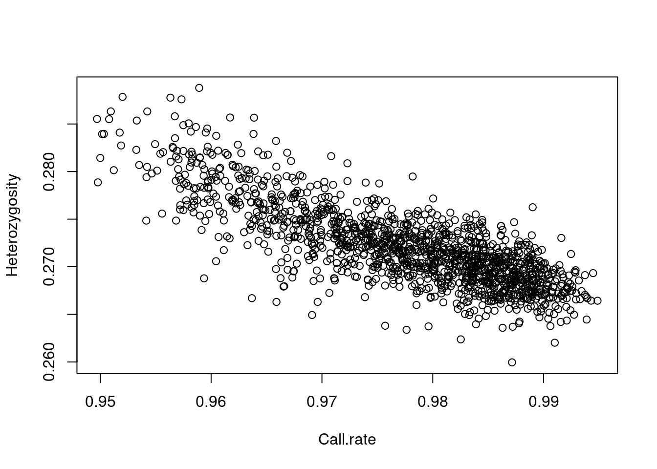

Past versions of snp-summary-1.png

Version	Author	Date
4e4427b	simingz	2024-01-02

Feel free to read the snpStats documentation and explore for yourself, but one standard thing that one is always interested in is to simply convert various SNPs to a regular numeric matrix so that you can analyze them using standard R tools. For example, let’s do a Fisher’s exact test to see whether CAD is associated with SNP 143:

x <- as(obj$genotypes[,143], 'numeric')
fisher.test(drop(x), as.factor(clinical$CAD))

    Fisher's Exact Test for Count Data

data:  drop(x) and as.factor(clinical$CAD)
p-value = 0.8043
alternative hypothesis: two.sided

Other R packages to read plink files.

There are several other R packages that can work with PLINK formatted files. - plink2R - pgenlibr, this package can work with plink2 formatted files, ie .pgen, pvar, psam. - bigsnpr

GWAS Quality Control (QC)

Check a few things. In actual GWAS, there are more to check.

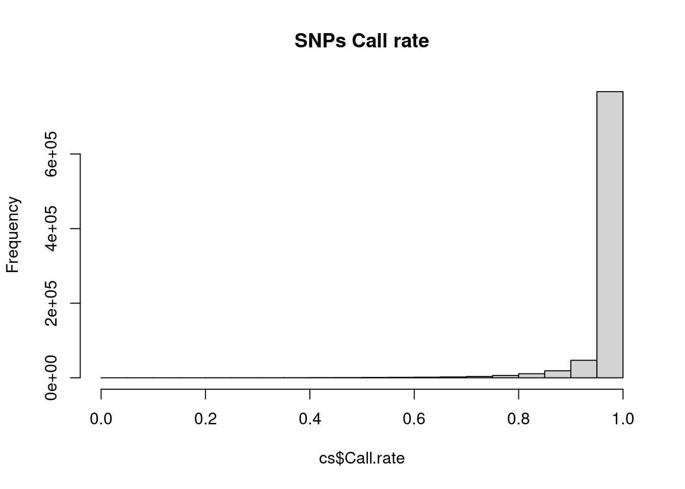
Any SNP with a lot of missing data is probably questionable; these SNPs are often excluded from analysis (although we will talk about other approaches later). Likewise, any sample with lots of missing data suggests that there may be issues with the processing of that sample.

cs <- col.summary(obj$genotypes)
rs <- row.summary(obj$genotypes)

hist(rs$Call.rate, main = 'Individuals Call rate')
hist(cs$Call.rate, main = 'SNPs Call rate')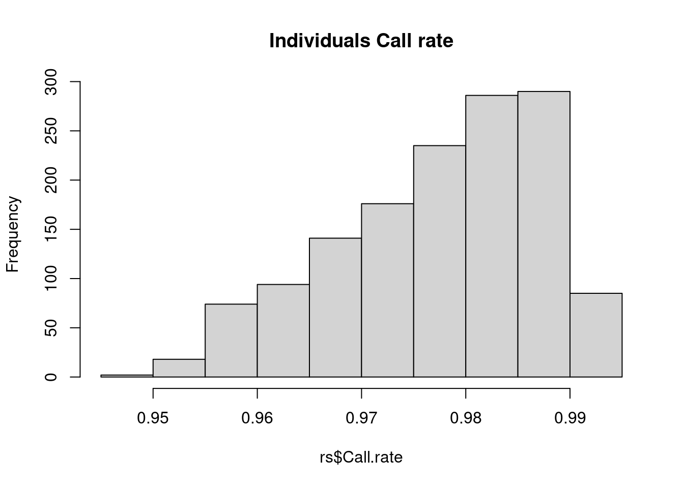

Past versions of miss-1.png

Version	Author	Date
4e4427b	simingz	2024-01-02

Past versions of miss-2.png

Version	Author	Date
4e4427b	simingz	2024-01-02

Individuals look good – SNPs, on the other hand, there are definitely some SNPs with lots of missing values. A common practice is to exclude SNPs with >5% or >10% missing data.

We will remove SNPs that may be problematic.

p_hwe <- 2*pnorm(-abs(cs$z.HWE)) # hardy-weinberg equilibrium. extreme value may indicate genotype error.

keep <- cs$MAF > 0.001 &
  cs$Call.rate > 0.9 & 
   abs(cs$z.HWE) < 6.5

(obj$genotypes <- obj$genotypes[, keep])

A SnpMatrix with  1401 rows and  752675 columns
Row names:  10002 ... 11596 
Col names:  rs12565286 ... rs28729663 

obj$map <- obj$map[keep, ]

# write plnik files for filtered data.
write.plink(
  file.base = "data/geno.qc",
  snps = obj$genotypes,
  pedigree = obj$fam$pedigree,
  id = obj$fam$member,
  father = obj$fam$father,
  mother = obj$fam$mother,
  chromosome = obj$map$chromosome,
  genetic.distance = obj$map$cM,
  position = obj$map$position,
  allele.1 = obj$map$allele.1,
  allele.2 = obj$map$allele.2,
  sex = clinical$sex,
  phenotype = clinical$CAD + 1
)

Writing FAM file to data/geno.qc.fam 
Writing extended MAP file to data/geno.qc.bim 
Writing BED file to data/geno.qc.bed (SNP-major mode)

NULL

Population structure.

It is possible to run PCA inside R, but given the large file size. Usually this is done by running plink from the command line.

Create a folder called output first.

plink -bfile data/geno.qc --pca --out output/pca

Then in R, we read in PCs and plot.

## read plink calculated PCs
pcplink = read.table("output/pca.eigenvec",header=F, as.is=T)
names(pcplink) = c("FID","IID",paste0("PC", c(1:(ncol(pcplink)-2))) )

## plot PC1 vs PC2
plot(pcplink$PC1, pcplink$PC2)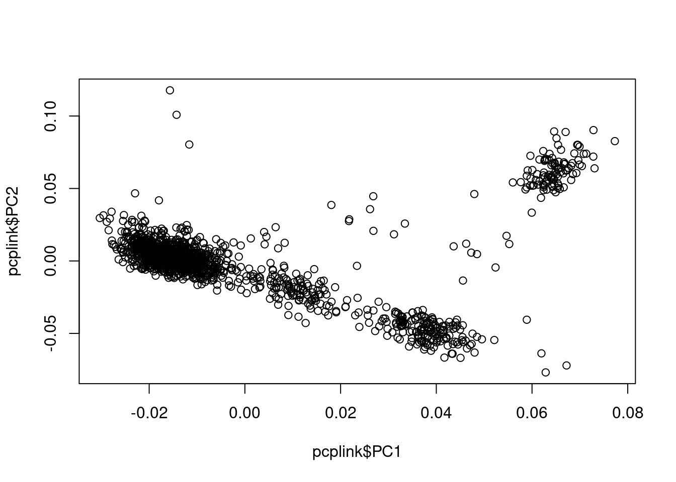

Past versions of PCA-1.png

Version	Author	Date
4e4427b	simingz	2024-01-02

## plot variance explained by PCs
eigen = read.table("output/pca.eigenval",header=F, as.is=T)[,1]
plot(1:length(eigen), eigen/nrow(pcplink), type = 'b', ylab = 'Proportion of variance explained', xlab = 'PC')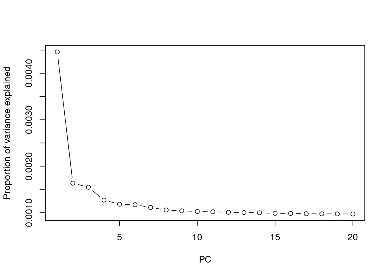

Past versions of PCA-2.png

Version	Author	Date
4e4427b	simingz	2024-01-02

Association testing

Run logistic regression using plink, adjusting for PCs. We will need to modify the original penncath.csv a bit to conform with plink phenotype file format:

clinical <- data.table::fread('data/penncath.csv', header = T)
colnames(clinical)[1] <- "FID"  # the first two column names have to be "FID and "IID" to serve as phenotype files for plink
clinical$IID <- 1
clinical <- clinical[, c("FID", "IID", "CAD", "sex", "age","tg","hdl","ldl")]
clinical$CAD <- clinical$CAD + 1 # in plink phenotype file, 0 is missing value, 2 is case, 1 is control for case-control study design.
write.table(clinical, file = "data/penncath4plink.csv", row.names = F, col.names = T, quote = F)
head(clinical)

     FID IID CAD sex age  tg hdl ldl
1: 10002   1   2   1  60  NA  NA  NA
2: 10004   1   2   2  50  55  23  75
3: 10005   1   2   1  55 105  37  69
4: 10007   1   2   1  52 314  54 108
5: 10008   1   2   1  58 161  40  94
6: 10009   1   2   1  59 171  46  92

Run the following from command line.

plink --bfile data/geno.qc --logistic --pheno data/penncath4plink.csv --pheno-name CAD --covar output/pca.eigenvec --covar-number 1-4 --out output/asso

Read results into R and plot

res <- fread('output/asso.assoc.logistic')
res <- res[res$TEST == "ADD",]
source("code/qqunif.R")
qqunif(res$P, mlog10_p_thres=12)

Warning in qqunif(res$P, mlog10_p_thres = 12): thresholding p to 1e-12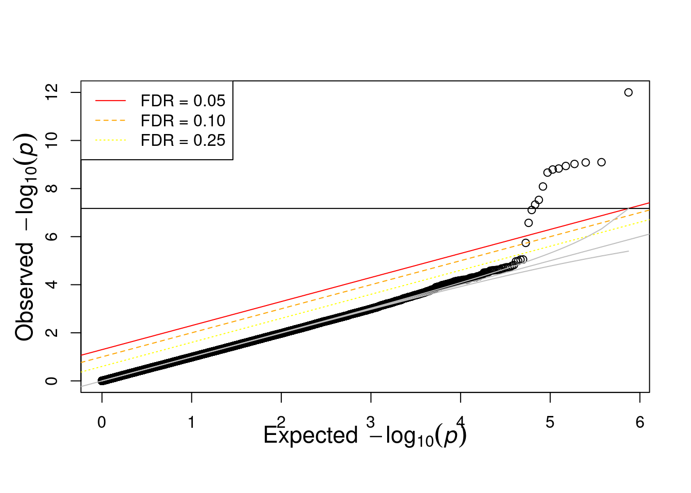

Past versions of plotres-1.png

Version	Author	Date
4e4427b	simingz	2024-01-02

Manhattan plot.

bim <- fread('data/geno.qc.bim')
# format data to have readable labels. 
manh_data <- data.frame(
    SNP = res$SNP,
    P = res$P
  ) %>%
  left_join(bim, by = c("SNP" = "V2")) %>%
  rename(
    CHR = V1, 
    BP = V4
  ) # recall that 'bim' files have a standardized format, so the column order is 
# always the same 
library(qqman)

For example usage please run: vignette('qqman')

Citation appreciated but not required:

Turner, (2018). qqman: an R package for visualizing GWAS results using Q-Q and manhattan plots. Journal of Open Source Software, 3(25), 731, https://doi.org/10.21105/joss.00731.

manh_plot <- manhattan(manh_data, ylim = c(0, 10), annotatePval = 5e-6)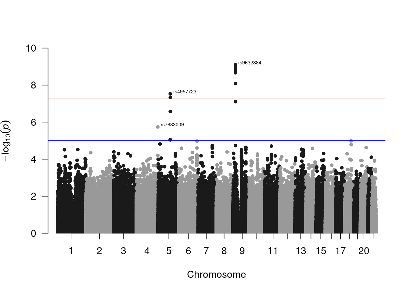

Past versions of plotmanh-1.png

Version	Author	Date
4e4427b	simingz	2024-01-02

Citation

Credits go to: https://github.com/pbreheny/adv-gwas-tutorial/tree/master.
https://yosuketanigawa.com/posts/2020/09/PLINK2
https://hakyimlab.github.io/hgen471/L6-population-structure.html

Session information

sessionInfo()

R version 4.1.0 (2021-05-18)
Platform: x86_64-pc-linux-gnu (64-bit)
Running under: CentOS Linux 7 (Core)

Matrix products: default
BLAS:   /software/R-4.1.0-no-openblas-el7-x86_64/lib64/R/lib/libRblas.so
LAPACK: /software/R-4.1.0-no-openblas-el7-x86_64/lib64/R/lib/libRlapack.so

locale:
 [1] LC_CTYPE=en_US.UTF-8 LC_NUMERIC=C         LC_TIME=C           
 [4] LC_COLLATE=C         LC_MONETARY=C        LC_MESSAGES=C       
 [7] LC_PAPER=C           LC_NAME=C            LC_ADDRESS=C        
[10] LC_TELEPHONE=C       LC_MEASUREMENT=C     LC_IDENTIFICATION=C 

attached base packages:
[1] stats     graphics  grDevices utils     datasets  methods   base     

other attached packages:
[1] qqman_0.1.9       snpStats_1.44.0   Matrix_1.3-3      survival_3.2-11  
[5] dplyr_1.0.7       data.table_1.14.0

loaded via a namespace (and not attached):
 [1] tidyselect_1.1.1    xfun_0.38           bslib_0.4.2        
 [4] purrr_0.3.4         splines_4.1.0       lattice_0.20-44    
 [7] vctrs_0.3.8         generics_0.1.0      htmltools_0.5.5    
[10] yaml_2.2.1          utf8_1.2.1          rlang_1.1.0        
[13] jquerylib_0.1.4     later_1.2.0         pillar_1.6.1       
[16] glue_1.4.2          DBI_1.1.1           BiocGenerics_0.40.0
[19] calibrate_1.7.7     lifecycle_1.0.3     stringr_1.4.0      
[22] zlibbioc_1.40.0     workflowr_1.6.2     evaluate_0.20      
[25] knitr_1.42          fastmap_1.1.0       httpuv_1.6.1       
[28] fansi_0.5.0         highr_0.9           Rcpp_1.0.9         
[31] promises_1.2.0.1    cachem_1.0.5        jsonlite_1.7.2     
[34] fs_1.6.1            digest_0.6.27       stringi_1.6.2      
[37] rprojroot_2.0.2     grid_4.1.0          cli_3.6.1          
[40] tools_4.1.0         magrittr_2.0.1      sass_0.4.0         
[43] tibble_3.1.2        crayon_1.5.2        whisker_0.4        
[46] pkgconfig_2.0.3     MASS_7.3-54         ellipsis_0.3.2     
[49] assertthat_0.2.1    rmarkdown_2.21      rstudioapi_0.13    
[52] R6_2.5.0            git2r_0.28.0        compiler_4.1.0