Atrial fibrillation - Heart Atrial Appendage
sheng Qian
2021-12-18
Last updated: 2021-12-20
Checks: 7 0
Knit directory: cTWAS_analysis/
This reproducible R Markdown analysis was created with workflowr (version 1.6.2). The Checks tab describes the reproducibility checks that were applied when the results were created. The Past versions tab lists the development history.
Great! Since the R Markdown file has been committed to the Git repository, you know the exact version of the code that produced these results.
Great job! The global environment was empty. Objects defined in the global environment can affect the analysis in your R Markdown file in unknown ways. For reproduciblity it’s best to always run the code in an empty environment.
The command set.seed(20211220) was run prior to running the code in the R Markdown file. Setting a seed ensures that any results that rely on randomness, e.g. subsampling or permutations, are reproducible.
Great job! Recording the operating system, R version, and package versions is critical for reproducibility.
Nice! There were no cached chunks for this analysis, so you can be confident that you successfully produced the results during this run.
Great job! Using relative paths to the files within your workflowr project makes it easier to run your code on other machines.
Great! You are using Git for version control. Tracking code development and connecting the code version to the results is critical for reproducibility.
The results in this page were generated with repository version 12069cf. See the Past versions tab to see a history of the changes made to the R Markdown and HTML files.
Note that you need to be careful to ensure that all relevant files for the analysis have been committed to Git prior to generating the results (you can use wflow_publish or wflow_git_commit). workflowr only checks the R Markdown file, but you know if there are other scripts or data files that it depends on. Below is the status of the Git repository when the results were generated:
Untracked files:
    Untracked:  code/run_AF_analysis.sbatch
    Untracked:  code/run_AF_analysis.sh
    Untracked:  code/run_AF_ctwas_rss_LDR.R
    Untracked:  data/AF/
Note that any generated files, e.g. HTML, png, CSS, etc., are not included in this status report because it is ok for generated content to have uncommitted changes.
These are the previous versions of the repository in which changes were made to the R Markdown (analysis/Atrial_Fibrillation_Heart_Atrial_Appendage.Rmd) and HTML (docs/Atrial_Fibrillation_Heart_Atrial_Appendage.html) files. If you’ve configured a remote Git repository (see ?wflow_git_remote), click on the hyperlinks in the table below to view the files as they were in that past version.
| File | Version | Author | Date | Message |
|---|---|---|---|---|
| Rmd | 12069cf | sq-96 | 2021-12-20 | Publish the files |
qclist_all <- list()

qc_files <- paste0(results_dir, "/", list.files(results_dir, pattern="exprqc.Rd"))

for (i in 1:length(qc_files)){
  load(qc_files[i])
  chr <- unlist(strsplit(rev(unlist(strsplit(qc_files[i], "_")))[1], "[.]"))[1]
  qclist_all[[chr]] <- cbind(do.call(rbind, lapply(qclist,unlist)), as.numeric(substring(chr,4)))
}

qclist_all <- data.frame(do.call(rbind, qclist_all))
colnames(qclist_all)[ncol(qclist_all)] <- "chr"

rm(qclist, wgtlist, z_gene_chr)

#number of imputed weights
nrow(qclist_all)
[1] 10862#number of imputed weights by chromosome
table(qclist_all$chr)
   1    2    3    4    5    6    7    8    9   10   11   12   13   14   15   16
1103  776  625  427  501  624  518  377  399  423  648  611  203  368  356  495
  17   18   19   20   21   22
 676  177  840  318  126  271
#proportion of imputed weights without missing variants
mean(qclist_all$nmiss==0)[1] 0.6548518library(ggplot2)
library(cowplot)
********************************************************Note: As of version 1.0.0, cowplot does not change the default ggplot2 theme anymore. To recover the previous behavior, execute:
theme_set(theme_cowplot())********************************************************load(paste0(results_dir, "/", analysis_id, "_ctwas.s2.susieIrssres.Rd"))
df <- data.frame(niter = rep(1:ncol(group_prior_rec), 2),
value = c(group_prior_rec[1,], group_prior_rec[2,]),
group = rep(c("Gene", "SNP"), each = ncol(group_prior_rec)))
df$group <- as.factor(df$group)
df$value[df$group=="SNP"] <- df$value[df$group=="SNP"]*thin #adjust parameter to account for thin argument
p_pi <- ggplot(df, aes(x=niter, y=value, group=group)) +
geom_line(aes(color=group)) +
geom_point(aes(color=group)) +
xlab("Iteration") + ylab(bquote(pi)) +
ggtitle("Prior mean") +
theme_cowplot()
df <- data.frame(niter = rep(1:ncol(group_prior_var_rec), 2),
value = c(group_prior_var_rec[1,], group_prior_var_rec[2,]),
group = rep(c("Gene", "SNP"), each = ncol(group_prior_var_rec)))
df$group <- as.factor(df$group)
p_sigma2 <- ggplot(df, aes(x=niter, y=value, group=group)) +
geom_line(aes(color=group)) +
geom_point(aes(color=group)) +
xlab("Iteration") + ylab(bquote(sigma^2)) +
ggtitle("Prior variance") +
theme_cowplot()
plot_grid(p_pi, p_sigma2)
#estimated group prior
estimated_group_prior <- group_prior_rec[,ncol(group_prior_rec)]
names(estimated_group_prior) <- c("gene", "snp")
estimated_group_prior["snp"] <- estimated_group_prior["snp"]*thin #adjust parameter to account for thin argument
print(estimated_group_prior)
gene snp
0.0208487453 0.0001927855 #estimated group prior variance
estimated_group_prior_var <- group_prior_var_rec[,ncol(group_prior_var_rec)]
names(estimated_group_prior_var) <- c("gene", "snp")
print(estimated_group_prior_var) gene snp
9.646456 8.679052 #report sample size
print(sample_size)[1] 1030836#report group size
group_size <- c(nrow(ctwas_gene_res), n_snps)
print(group_size)[1] 10862 6839050#estimated group PVE
estimated_group_pve <- estimated_group_prior_var*estimated_group_prior*group_size/sample_size #check PVE calculation
names(estimated_group_pve) <- c("gene", "snp")
print(estimated_group_pve) gene snp
0.00211918 0.01110076 #compare sum(PIP*mu2/sample_size) with above PVE calculation
c(sum(ctwas_gene_res$PVE),sum(ctwas_snp_res$PVE))[1] 0.01225055 0.12523867#distribution of PIPs
hist(ctwas_gene_res$susie_pip, xlim=c(0,1), main="Distribution of Gene PIPs")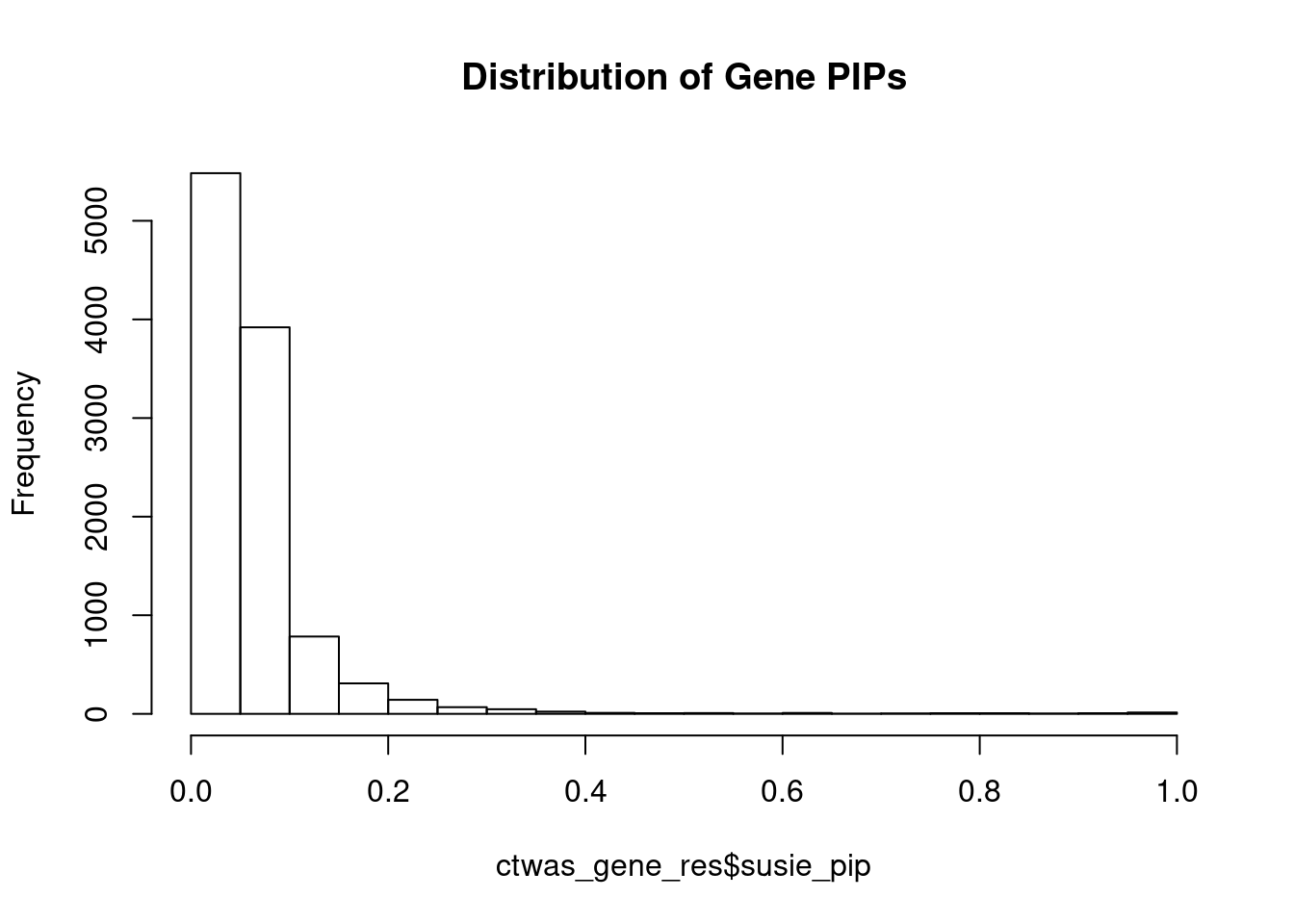
#genes with PIP>0.8 or 20 highest PIPs
head(ctwas_gene_res[order(-ctwas_gene_res$susie_pip),report_cols], max(sum(ctwas_gene_res$susie_pip>0.8), 20))
genename region_tag susie_pip mu2 PVE z
2293 CAV1 7_70 1.0000000 622.84815 6.042165e-04 15.567870
3275 PRRX1 1_84 0.9998808 119.34663 1.157627e-04 14.667578
4009 DEK 6_14 0.9925129 63.47784 6.111795e-05 -9.000000
3527 CCND2 12_4 0.9906174 27.01637 2.596231e-05 -5.283784
1310 PXN 12_75 0.9826498 29.47170 2.809405e-05 -5.328302
12836 RP11-325L7.2 5_82 0.9826020 1993.73789 1.900449e-03 12.356322
9257 AGAP5 10_49 0.9779202 48.91516 4.640420e-05 11.518590
3523 KLF12 13_36 0.9770829 26.00017 2.464439e-05 -5.072464
6621 AKAP6 14_8 0.9721549 76.81846 7.244551e-05 -9.197368
6914 JAM2 21_9 0.9640543 22.19279 2.075505e-05 4.563232
9639 DLEU1 13_21 0.9586468 23.59091 2.193885e-05 4.697095
11818 DPF3 14_34 0.9574312 33.35512 3.097993e-05 6.264960
10521 FAM43A 3_120 0.9569176 29.69898 2.756935e-05 -5.487179
2444 SEC23IP 10_74 0.9517809 22.38862 2.067163e-05 -4.565228
13075 LINC01629 14_36 0.9471613 31.88580 2.929757e-05 -5.695652
2138 AES 19_4 0.9403219 20.20438 1.843030e-05 4.182804
4658 POPDC3 6_70 0.9252511 25.19514 2.261449e-05 -4.758170
10290 NKX2-5 5_103 0.9228745 61.55975 5.511247e-05 -9.391892
7515 TNFSF13 17_7 0.9135188 34.26969 3.036953e-05 -5.883117
5185 GYPC 2_74 0.9068050 38.95864 3.427111e-05 -6.380531
8248 CMTM5 14_3 0.9067300 30.09803 2.647442e-05 -5.472727
10548 SCN10A 3_28 0.8867624 77.72022 6.685774e-05 -8.814286
13967 RP5-890E16.5 17_28 0.8660551 23.11200 1.941751e-05 -4.761194
712 SP100 2_135 0.8658723 18.73540 1.573719e-05 -3.671335
9012 MTSS1 8_82 0.8594108 20.87861 1.740655e-05 4.402634
8992 MURC 9_50 0.8478869 23.34736 1.920376e-05 4.911964
5223 PSMB7 9_64 0.8430652 25.30057 2.069197e-05 -4.820896
6114 STK11IP 2_130 0.8406381 18.96825 1.546845e-05 -3.868022
10416 PGP 16_2 0.8298586 28.51218 2.295329e-05 5.943820
9691 BOK 2_144 0.8255975 19.18259 1.536335e-05 3.910125
8420 MARS 12_36 0.8180336 17.81958 1.414097e-05 -3.366197
3088 GNB4 3_110 0.8097696 30.34628 2.383842e-05 -5.583333
num_eqtl
2293 3
3275 2
4009 1
3527 1
1310 1
12836 1
9257 2
3523 1
6621 1
6914 2
9639 1
11818 3
10521 1
2444 2
13075 1
2138 3
4658 1
10290 1
7515 1
5185 1
8248 1
10548 1
13967 1
712 2
9012 2
8992 2
5223 1
6114 2
10416 1
9691 3
8420 1
3088 1Genes with largest effect sizes
#plot PIP vs effect size
plot(ctwas_gene_res$susie_pip, ctwas_gene_res$mu2, xlab="PIP", ylab="mu^2", main="Gene PIPs vs Effect Size")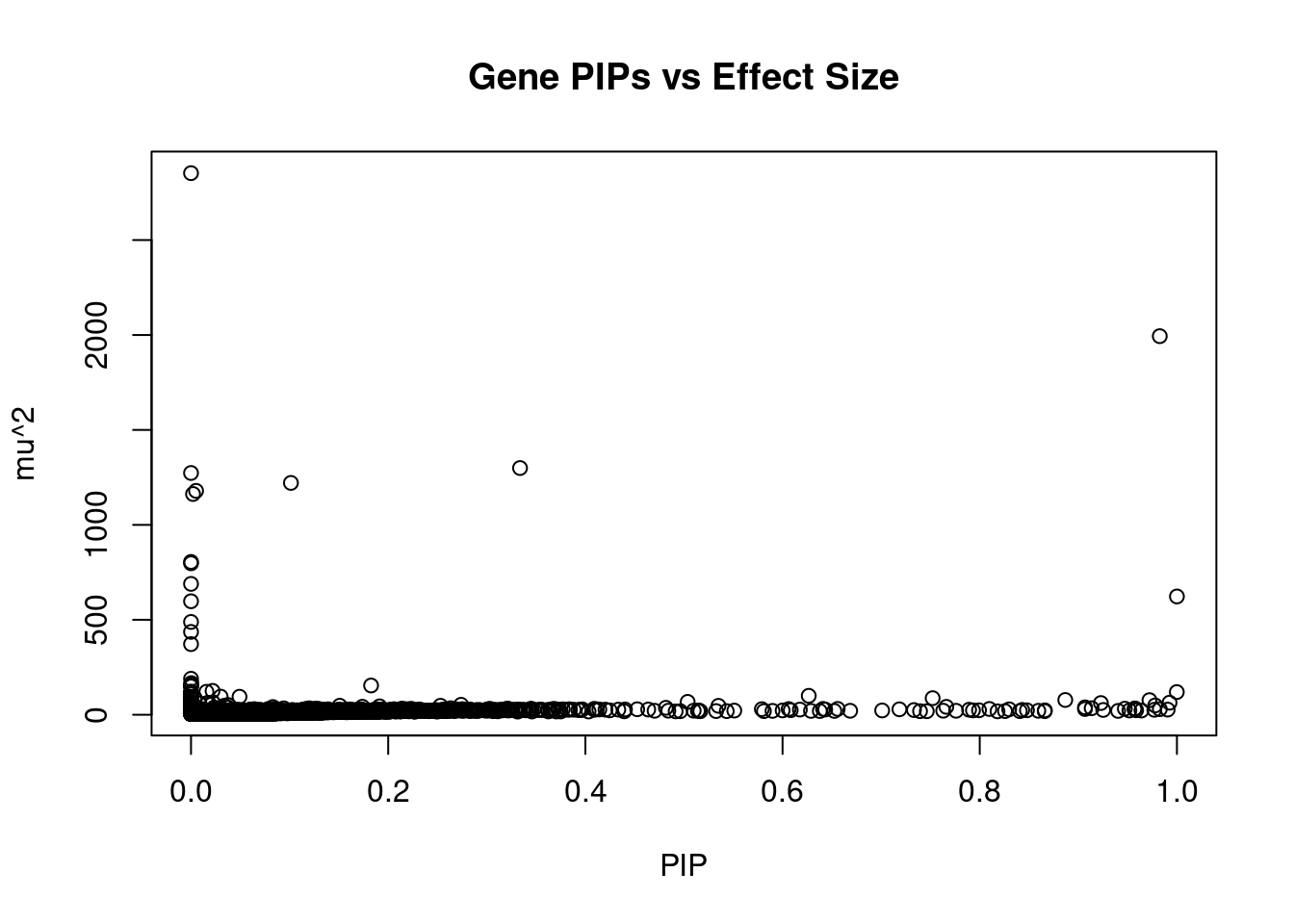
#genes with 20 largest effect sizes
head(ctwas_gene_res[order(-ctwas_gene_res$mu2),report_cols],10)
genename region_tag susie_pip mu2 PVE z
3250 WIPF1 2_105 0.000000e+00 2852.2491 0.000000e+00 8.441558
12836 RP11-325L7.2 5_82 9.826020e-01 1993.7379 1.900449e-03 12.356322
1487 SIRT1 10_44 3.337242e-01 1299.2406 4.206179e-04 -5.053846
7413 IL6R 1_75 5.862422e-12 1273.1807 7.240649e-15 -4.978495
6444 HERC4 10_44 1.013394e-01 1220.9395 1.200281e-04 -5.359560
11106 NACA 12_35 5.127731e-03 1179.0569 5.865032e-06 -6.240809
960 BAZ2A 12_35 2.047295e-03 1162.5562 2.308898e-06 -5.942857
7986 SLC35A1 6_59 0.000000e+00 804.8763 0.000000e+00 -5.072464
2507 WNT3 17_27 3.707228e-05 797.4584 2.867925e-08 -4.389402
2292 CAV2 7_70 0.000000e+00 689.1121 0.000000e+00 14.534943
num_eqtl
3250 1
12836 1
1487 1
7413 1
6444 2
11106 2
960 1
7986 1
2507 2
2292 2Genes with highest PVE
#genes with 20 highest pve
head(ctwas_gene_res[order(-ctwas_gene_res$PVE),report_cols],10)
genename region_tag susie_pip mu2 PVE z
12836 RP11-325L7.2 5_82 0.9826020 1993.73789 1.900449e-03 12.356322
2293 CAV1 7_70 1.0000000 622.84815 6.042165e-04 15.567870
1487 SIRT1 10_44 0.3337242 1299.24064 4.206179e-04 -5.053846
6444 HERC4 10_44 0.1013394 1220.93950 1.200281e-04 -5.359560
3275 PRRX1 1_84 0.9998808 119.34663 1.157627e-04 14.667578
6621 AKAP6 14_8 0.9721549 76.81846 7.244551e-05 -9.197368
10548 SCN10A 3_28 0.8867624 77.72022 6.685774e-05 -8.814286
12013 ZSWIM8 10_49 0.7522384 87.25963 6.367652e-05 -11.216495
4009 DEK 6_14 0.9925129 63.47784 6.111795e-05 -9.000000
8298 SYNPO2L 10_49 0.6265676 99.72467 6.061512e-05 -11.945652
num_eqtl
12836 1
2293 3
1487 1
6444 2
3275 2
6621 1
10548 1
12013 1
4009 1
8298 1Genes with largest z scores
#genes with 20 largest z scores
head(ctwas_gene_res[order(-abs(ctwas_gene_res$z)),report_cols],10)
genename region_tag susie_pip mu2 PVE z
2293 CAV1 7_70 1.000000e+00 622.84815 6.042165e-04 15.56787
3275 PRRX1 1_84 9.998808e-01 119.34663 1.157627e-04 14.66758
2292 CAV2 7_70 0.000000e+00 689.11215 0.000000e+00 14.53494
12836 RP11-325L7.2 5_82 9.826020e-01 1993.73789 1.900449e-03 12.35632
7729 PMVK 1_76 9.693335e-05 161.14638 1.515319e-08 -12.10294
8298 SYNPO2L 10_49 6.265676e-01 99.72467 6.061512e-05 -11.94565
7730 PBXIP1 1_76 9.335873e-05 156.14141 1.414111e-08 -11.86765
9805 MYOZ1 10_49 3.497772e-03 88.98387 3.019349e-07 11.75935
9257 AGAP5 10_49 9.779202e-01 48.91516 4.640420e-05 11.51859
12013 ZSWIM8 10_49 7.522384e-01 87.25963 6.367652e-05 -11.21649
num_eqtl
2293 3
3275 2
2292 2
12836 1
7729 1
8298 1
7730 1
9805 2
9257 2
12013 1Comparing z scores and PIPs
#set nominal signifiance threshold for z scores
alpha <- 0.05

#bonferroni adjusted threshold for z scores
sig_thresh <- qnorm(1-(alpha/nrow(ctwas_gene_res)/2), lower=T)

#Q-Q plot for z scores
obs_z <- ctwas_gene_res$z[order(ctwas_gene_res$z)]
exp_z <- qnorm((1:nrow(ctwas_gene_res))/nrow(ctwas_gene_res))

plot(exp_z, obs_z, xlab="Expected z", ylab="Observed z", main="Gene z score Q-Q plot")
abline(a=0,b=1)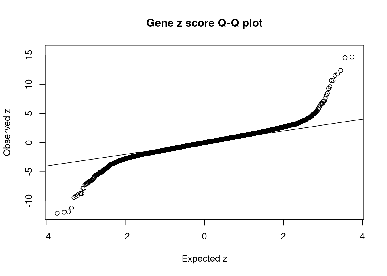
#plot z score vs PIP
plot(abs(ctwas_gene_res$z), ctwas_gene_res$susie_pip, xlab="abs(z)", ylab="PIP")
abline(v=sig_thresh, col="red", lty=2)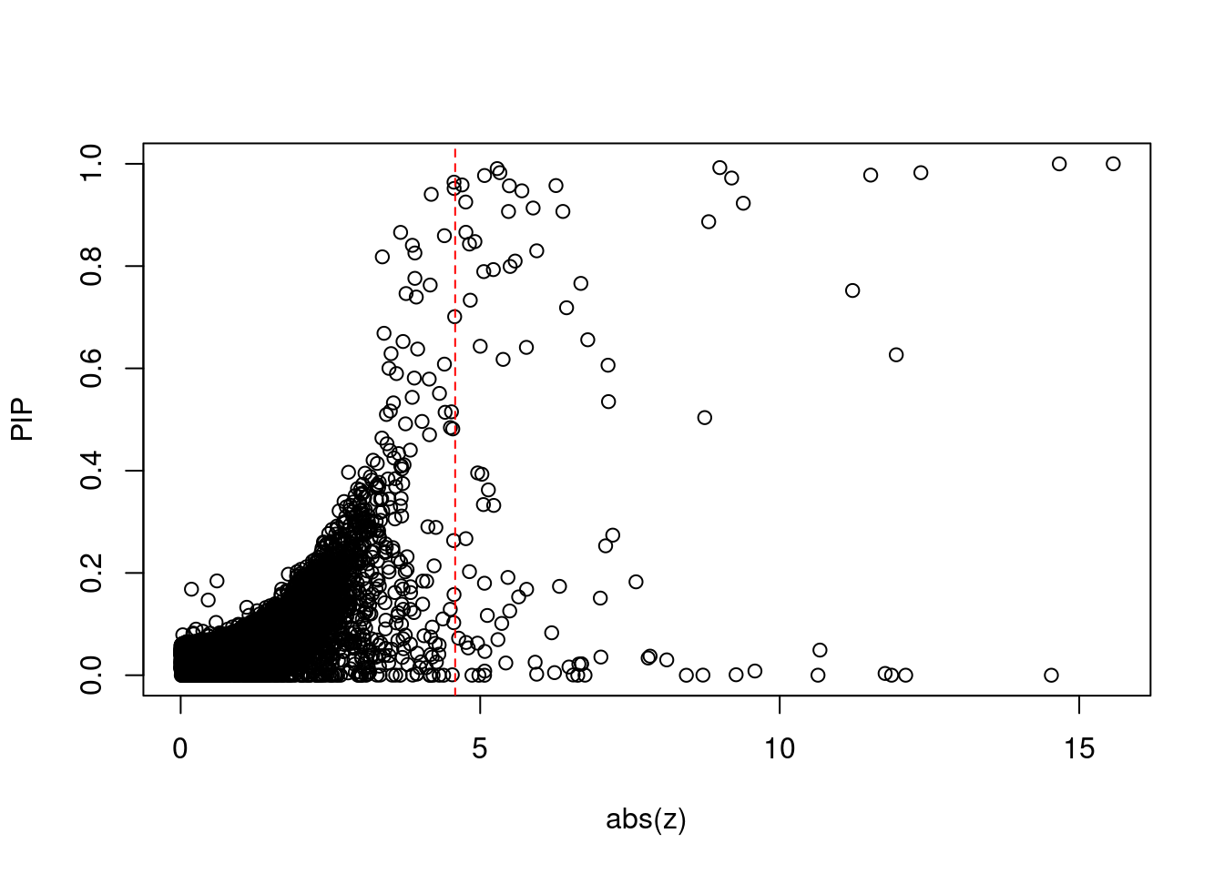
#proportion of significant z scores
mean(abs(ctwas_gene_res$z) > sig_thresh)
[1] 0.008654023#genes with most significant z scores
head(ctwas_gene_res[order(-abs(ctwas_gene_res$z)),report_cols],20) genename region_tag susie_pip mu2 PVE z
2293 CAV1 7_70 1.000000e+00 622.84815 6.042165e-04 15.567870
3275 PRRX1 1_84 9.998808e-01 119.34663 1.157627e-04 14.667578
2292 CAV2 7_70 0.000000e+00 689.11215 0.000000e+00 14.534943
12836 RP11-325L7.2 5_82 9.826020e-01 1993.73789 1.900449e-03 12.356322
7729 PMVK 1_76 9.693335e-05 161.14638 1.515319e-08 -12.102941
8298 SYNPO2L 10_49 6.265676e-01 99.72467 6.061512e-05 -11.945652
7730 PBXIP1 1_76 9.335873e-05 156.14141 1.414111e-08 -11.867647
9805 MYOZ1 10_49 3.497772e-03 88.98387 3.019349e-07 11.759348
9257 AGAP5 10_49 9.779202e-01 48.91516 4.640420e-05 11.518590
12013 ZSWIM8 10_49 7.522384e-01 87.25963 6.367652e-05 -11.216495
6395 C9orf3 9_48 4.919856e-02 94.74228 4.521751e-06 10.671642
7407 ZBTB7B 1_76 9.636563e-05 122.09475 1.141378e-08 10.638889
13556 RP1-79C4.4 1_84 8.254209e-03 58.95140 4.720414e-07 9.586404
10290 NKX2-5 5_103 9.228745e-01 61.55975 5.511247e-05 -9.391892
9719 SEC24C 10_49 9.597200e-04 46.26092 4.306945e-08 9.271945
6621 AKAP6 14_8 9.721549e-01 76.81846 7.244551e-05 -9.197368
4009 DEK 6_14 9.925129e-01 63.47784 6.111795e-05 -9.000000
10548 SCN10A 3_28 8.867624e-01 77.72022 6.685774e-05 -8.814286
3665 KCNJ5 11_80 5.037532e-01 67.73277 3.309993e-05 -8.748092
7733 DCST2 1_76 2.613168e-04 89.76014 2.275418e-08 -8.718310
num_eqtl
2293 3
3275 2
2292 2
12836 1
7729 1
8298 1
7730 1
9805 2
9257 2
12013 1
6395 1
7407 1
13556 2
10290 1
9719 2
6621 1
4009 1
10548 1
3665 1
7733 1library(tibble)
library(tidyverse)── Attaching packages ─────────────────────────────────────── tidyverse 1.3.1 ──✔ tidyr 1.1.4 ✔ dplyr 1.0.7
✔ readr 2.1.1 ✔ stringr 1.4.0
✔ purrr 0.3.4 ✔ forcats 0.5.1── Conflicts ────────────────────────────────────────── tidyverse_conflicts() ──
✖ dplyr::filter() masks stats::filter()
✖ dplyr::lag() masks stats::lag()full.gene.pip.summary <- data.frame(gene_name = ctwas_gene_res$genename,
gene_pip = ctwas_gene_res$susie_pip,
gene_id = ctwas_gene_res$id,
chr = as.integer(ctwas_gene_res$chrom),
start = ctwas_gene_res$pos / 1e3,
is_highlight = F, stringsAsFactors = F) %>% as_tibble()
full.gene.pip.summary$is_highlight <- full.gene.pip.summary$gene_pip > 0.80
don <- full.gene.pip.summary %>%
# Compute chromosome size
group_by(chr) %>%
summarise(chr_len=max(start)) %>%
# Calculate cumulative position of each chromosome
mutate(tot=cumsum(chr_len)-chr_len) %>%
dplyr::select(-chr_len) %>%
# Add this info to the initial dataset
left_join(full.gene.pip.summary, ., by=c("chr"="chr")) %>%
# Add a cumulative position of each SNP
arrange(chr, start) %>%
mutate( BPcum=start+tot)
axisdf <- don %>% group_by(chr) %>% summarize(center=( max(BPcum) + min(BPcum) ) / 2 )
x_axis_labels <- axisdf$chr
x_axis_labels[seq(1,21,2)] <- ""
ggplot(don, aes(x=BPcum, y=gene_pip)) +
# Show all points
ggrastr::geom_point_rast(aes(color=as.factor(chr)), size=2) +
scale_color_manual(values = rep(c("grey", "skyblue"), 22 )) +
# custom X axis:
# scale_x_continuous(label = axisdf$chr,
# breaks= axisdf$center,
# guide = guide_axis(n.dodge = 2)) +
scale_x_continuous(label = x_axis_labels,
breaks = axisdf$center) +
scale_y_continuous(expand = c(0, 0), limits = c(0,1.25), breaks=(1:5)*0.2, minor_breaks=(1:10)*0.1) + # remove space between plot area and x axis
# Add highlighted points
ggrastr::geom_point_rast(data=subset(don, is_highlight==T), color="orange", size=2) +
# Add label using ggrepel to avoid overlapping
ggrepel::geom_label_repel(data=subset(don, is_highlight==T),
aes(label=gene_name),
size=4,
min.segment.length = 0,
label.size = NA,
fill = alpha(c("white"),0)) +
# Custom the theme:
theme_bw() +
theme(
text = element_text(size = 14),
legend.position="none",
panel.border = element_blank(),
panel.grid.major.x = element_blank(),
panel.grid.minor.x = element_blank()
) +
xlab("Chromosome") +
ylab("cTWAS PIP")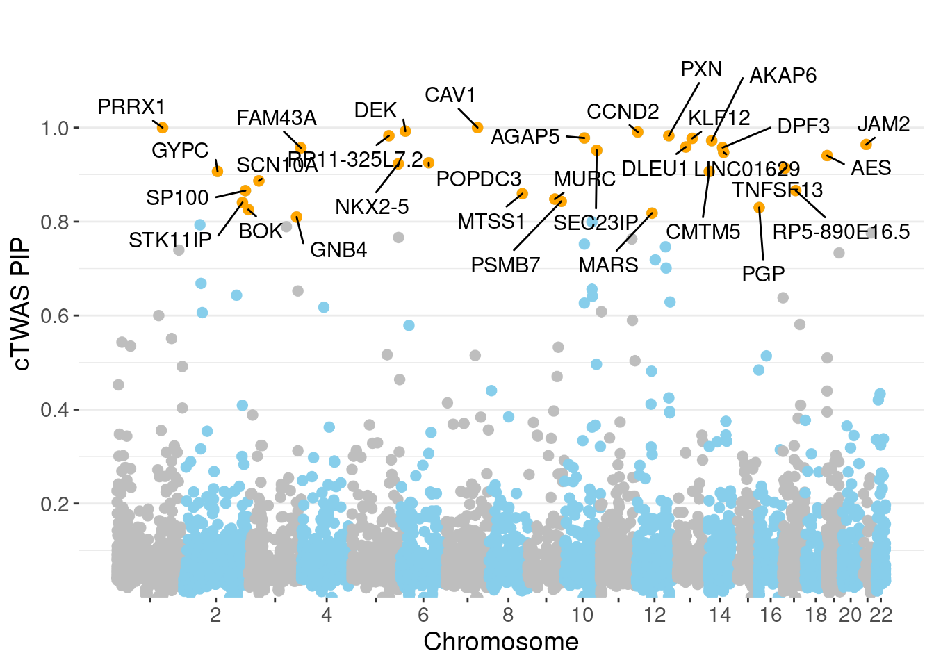
sessionInfo()R version 3.6.1 (2019-07-05)
Platform: x86_64-pc-linux-gnu (64-bit)
Running under: Scientific Linux 7.4 (Nitrogen)
Matrix products: default
BLAS/LAPACK: /software/openblas-0.2.19-el7-x86_64/lib/libopenblas_haswellp-r0.2.19.so
locale:
[1] LC_CTYPE=en_US.UTF-8 LC_NUMERIC=C
[3] LC_TIME=en_US.UTF-8 LC_COLLATE=en_US.UTF-8
[5] LC_MONETARY=en_US.UTF-8 LC_MESSAGES=en_US.UTF-8
[7] LC_PAPER=en_US.UTF-8 LC_NAME=C
[9] LC_ADDRESS=C LC_TELEPHONE=C
[11] LC_MEASUREMENT=en_US.UTF-8 LC_IDENTIFICATION=C
attached base packages:
[1] stats graphics grDevices utils datasets methods base
other attached packages:
[1] forcats_0.5.1 stringr_1.4.0 dplyr_1.0.7 purrr_0.3.4
[5] readr_2.1.1 tidyr_1.1.4 tidyverse_1.3.1 tibble_3.1.6
[9] cowplot_1.0.0 ggplot2_3.3.5 workflowr_1.6.2
loaded via a namespace (and not attached):
[1] httr_1.4.2 bit64_4.0.5 jsonlite_1.7.2 modelr_0.1.8
[5] assertthat_0.2.1 highr_0.9 blob_1.2.2 vipor_0.4.5
[9] cellranger_1.1.0 yaml_2.2.1 ggrepel_0.8.1 pillar_1.6.4
[13] RSQLite_2.2.8 backports_1.4.1 glue_1.5.1 digest_0.6.29
[17] promises_1.0.1 rvest_1.0.2 colorspace_2.0-2 htmltools_0.5.2
[21] httpuv_1.5.1 pkgconfig_2.0.3 broom_0.7.10 haven_2.4.3
[25] scales_1.1.1 whisker_0.3-2 ggrastr_1.0.1 later_0.8.0
[29] tzdb_0.2.0 git2r_0.26.1 generics_0.1.1 farver_2.1.0
[33] ellipsis_0.3.2 cachem_1.0.6 withr_2.4.3 cli_3.1.0
[37] magrittr_2.0.1 crayon_1.4.2 readxl_1.3.1 memoise_2.0.1
[41] evaluate_0.14 fs_1.5.2 fansi_0.5.0 xml2_1.3.3
[45] beeswarm_0.2.3 Cairo_1.5-12.2 tools_3.6.1 data.table_1.14.2
[49] hms_1.1.1 lifecycle_1.0.1 munsell_0.5.0 reprex_2.0.1
[53] compiler_3.6.1 jquerylib_0.1.4 rlang_0.4.12 grid_3.6.1
[57] rstudioapi_0.13 labeling_0.4.2 rmarkdown_2.11 gtable_0.3.0
[61] DBI_1.1.1 R6_2.5.1 lubridate_1.8.0 knitr_1.36
[65] fastmap_1.1.0 bit_4.0.4 utf8_1.2.2 rprojroot_2.0.2
[69] stringi_1.7.6 ggbeeswarm_0.6.0 Rcpp_1.0.7 vctrs_0.3.8
[73] dbplyr_2.1.1 tidyselect_1.1.1 xfun_0.29