SCZ - Brain Hypothalamus
sheng Qian
2021-2-6
Last updated: 2022-04-19
Checks: 5 2
Knit directory: cTWAS_analysis/
This reproducible R Markdown analysis was created with workflowr (version 1.7.0). The Checks tab describes the reproducibility checks that were applied when the results were created. The Past versions tab lists the development history.
The R Markdown file has unstaged changes. To know which version of the R Markdown file created these results, you’ll want to first commit it to the Git repo. If you’re still working on the analysis, you can ignore this warning. When you’re finished, you can run wflow_publish to commit the R Markdown file and build the HTML.
Great job! The global environment was empty. Objects defined in the global environment can affect the analysis in your R Markdown file in unknown ways. For reproduciblity it’s best to always run the code in an empty environment.
The command set.seed(20211220) was run prior to running the code in the R Markdown file. Setting a seed ensures that any results that rely on randomness, e.g. subsampling or permutations, are reproducible.
Great job! Recording the operating system, R version, and package versions is critical for reproducibility.
Nice! There were no cached chunks for this analysis, so you can be confident that you successfully produced the results during this run.
Using absolute paths to the files within your workflowr project makes it difficult for you and others to run your code on a different machine. Change the absolute path(s) below to the suggested relative path(s) to make your code more reproducible.
| absolute | relative |
|---|---|
| /project2/xinhe/shengqian/cTWAS/cTWAS_analysis/data/ | data |
| /project2/xinhe/shengqian/cTWAS/cTWAS_analysis/code/ctwas_config.R | code/ctwas_config.R |
Great! You are using Git for version control. Tracking code development and connecting the code version to the results is critical for reproducibility.
The results in this page were generated with repository version ba919ab. See the Past versions tab to see a history of the changes made to the R Markdown and HTML files.
Note that you need to be careful to ensure that all relevant files for the analysis have been committed to Git prior to generating the results (you can use wflow_publish or wflow_git_commit). workflowr only checks the R Markdown file, but you know if there are other scripts or data files that it depends on. Below is the status of the Git repository when the results were generated:
Ignored files:
    Ignored:    .ipynb_checkpoints/
    Ignored:    data/AF/

Untracked files:
    Untracked:  Rplot.png
    Untracked:  analysis/.ipynb_checkpoints/
    Untracked:  code/.ipynb_checkpoints/
    Untracked:  code/AF_out/
    Untracked:  code/Autism_out/
    Untracked:  code/BMI_S_out/
    Untracked:  code/BMI_out/
    Untracked:  code/Glucose_out/
    Untracked:  code/LDL_S_out/
    Untracked:  code/SCZ_2014_EUR_out/
    Untracked:  code/SCZ_2018_out/
    Untracked:  code/SCZ_2020_Single_out/
    Untracked:  code/SCZ_2020_out/
    Untracked:  code/SCZ_S_out/
    Untracked:  code/SCZ_out/
    Untracked:  code/T2D_out/
    Untracked:  code/ctwas_config.R
    Untracked:  code/mapping.R
    Untracked:  code/out/
    Untracked:  code/process_scz_2018_snps.R
    Untracked:  code/run_AF_analysis.sbatch
    Untracked:  code/run_AF_analysis.sh
    Untracked:  code/run_AF_ctwas_rss_LDR.R
    Untracked:  code/run_Autism_analysis.sbatch
    Untracked:  code/run_Autism_analysis.sh
    Untracked:  code/run_Autism_ctwas_rss_LDR.R
    Untracked:  code/run_BMI_analysis.sbatch
    Untracked:  code/run_BMI_analysis.sh
    Untracked:  code/run_BMI_analysis_S.sbatch
    Untracked:  code/run_BMI_analysis_S.sh
    Untracked:  code/run_BMI_ctwas_rss_LDR.R
    Untracked:  code/run_BMI_ctwas_rss_LDR_S.R
    Untracked:  code/run_Glucose_analysis.sbatch
    Untracked:  code/run_Glucose_analysis.sh
    Untracked:  code/run_Glucose_ctwas_rss_LDR.R
    Untracked:  code/run_LDL_analysis_S.sbatch
    Untracked:  code/run_LDL_analysis_S.sh
    Untracked:  code/run_LDL_ctwas_rss_LDR_S.R
    Untracked:  code/run_SCZ_2014_EUR_analysis.sbatch
    Untracked:  code/run_SCZ_2014_EUR_analysis.sh
    Untracked:  code/run_SCZ_2014_EUR_ctwas_rss_LDR.R
    Untracked:  code/run_SCZ_2018_analysis.sbatch
    Untracked:  code/run_SCZ_2018_analysis.sh
    Untracked:  code/run_SCZ_2018_ctwas_rss_LDR.R
    Untracked:  code/run_SCZ_2020_Single_analysis.sbatch
    Untracked:  code/run_SCZ_2020_Single_analysis.sh
    Untracked:  code/run_SCZ_2020_Single_ctwas_rss_LDR.R
    Untracked:  code/run_SCZ_2020_analysis.sbatch
    Untracked:  code/run_SCZ_2020_analysis.sh
    Untracked:  code/run_SCZ_2020_ctwas_rss_LDR.R
    Untracked:  code/run_SCZ_analysis.sbatch
    Untracked:  code/run_SCZ_analysis.sh
    Untracked:  code/run_SCZ_analysis_S.sbatch
    Untracked:  code/run_SCZ_analysis_S.sh
    Untracked:  code/run_SCZ_ctwas_rss_LDR.R
    Untracked:  code/run_SCZ_ctwas_rss_LDR_S.R
    Untracked:  code/run_T2D_analysis.sbatch
    Untracked:  code/run_T2D_analysis.sh
    Untracked:  code/run_T2D_ctwas_rss_LDR.R
    Untracked:  code/wflow_build.R
    Untracked:  code/wflow_build.sbatch
    Untracked:  data/.ipynb_checkpoints/
    Untracked:  data/BMI/
    Untracked:  data/GO_Terms/
    Untracked:  data/PGC3_SCZ_wave3_public.v2.tsv
    Untracked:  data/SCZ/
    Untracked:  data/SCZ_2014_EUR/
    Untracked:  data/SCZ_2018/
    Untracked:  data/SCZ_2020/
    Untracked:  data/SCZ_2020_Single/
    Untracked:  data/SCZ_S/
    Untracked:  data/Supplementary Table 15 - MAGMA.xlsx
    Untracked:  data/Supplementary Table 20 - Prioritised Genes.xlsx
    Untracked:  data/T2D/
    Untracked:  data/UKBB/
    Untracked:  data/UKBB_SNPs_Info.text
    Untracked:  data/gene_OMIM.txt
    Untracked:  data/gene_pip_0.8.txt
    Untracked:  data/mashr_Heart_Atrial_Appendage.db
    Untracked:  data/mashr_sqtl/
    Untracked:  data/scz_2018.RDS
    Untracked:  data/summary_known_genes_annotations.xlsx
    Untracked:  data/untitled.txt
    Untracked:  top_genes_32.txt
    Untracked:  top_genes_37.txt
    Untracked:  top_genes_43.txt
    Untracked:  top_genes_81.txt

Unstaged changes:
    Modified:   analysis/SCZ_2018_Brain_Amygdala.Rmd
    Modified:   analysis/SCZ_2018_Brain_Anterior_cingulate_cortex_BA24.Rmd
    Modified:   analysis/SCZ_2018_Brain_Caudate_basal_ganglia.Rmd
    Modified:   analysis/SCZ_2018_Brain_Cerebellar_Hemisphere.Rmd
    Modified:   analysis/SCZ_2018_Brain_Cerebellum.Rmd
    Modified:   analysis/SCZ_2018_Brain_Cortex.Rmd
    Modified:   analysis/SCZ_2018_Brain_Frontal_Cortex_BA9.Rmd
    Modified:   analysis/SCZ_2018_Brain_Hippocampus.Rmd
    Modified:   analysis/SCZ_2018_Brain_Hypothalamus.Rmd
    Modified:   analysis/SCZ_2018_Brain_Nucleus_accumbens_basal_ganglia.Rmd
    Modified:   analysis/SCZ_2018_Brain_Putamen_basal_ganglia.Rmd
    Modified:   analysis/SCZ_2018_Brain_Spinal_cord_cervical_c-1.Rmd
    Modified:   analysis/SCZ_2018_Brain_Substantia_nigra.Rmd
    Modified:   analysis/SCZ_Annotation_Analysis.Rmd
Note that any generated files, e.g. HTML, png, CSS, etc., are not included in this status report because it is ok for generated content to have uncommitted changes.
These are the previous versions of the repository in which changes were made to the R Markdown (analysis/SCZ_2018_Brain_Hypothalamus.Rmd) and HTML (docs/SCZ_2018_Brain_Hypothalamus.html) files. If you’ve configured a remote Git repository (see ?wflow_git_remote), click on the hyperlinks in the table below to view the files as they were in that past version.
| File | Version | Author | Date | Message |
|---|---|---|---|---|
| Rmd | 9ddc9c4 | sq-96 | 2022-04-18 | update |
| Rmd | f6e7062 | sq-96 | 2022-04-17 | update |
| html | f6e7062 | sq-96 | 2022-04-17 | update |
Weight QC
#number of imputed weights
nrow(qclist_all)
[1] 9567#number of imputed weights by chromosome
table(qclist_all$chr)
  1   2   3   4   5   6   7   8   9  10  11  12  13  14  15  16  17  18  19  20
943 663 573 390 482 553 471 366 357 395 569 552 184 321 332 385 578 154 739 282
 21  22
 30 248
#number of imputed weights without missing variants
sum(qclist_all$nmiss==0)[1] 6811#proportion of imputed weights without missing variants
mean(qclist_all$nmiss==0)[1] 0.7119Check convergence of parameters
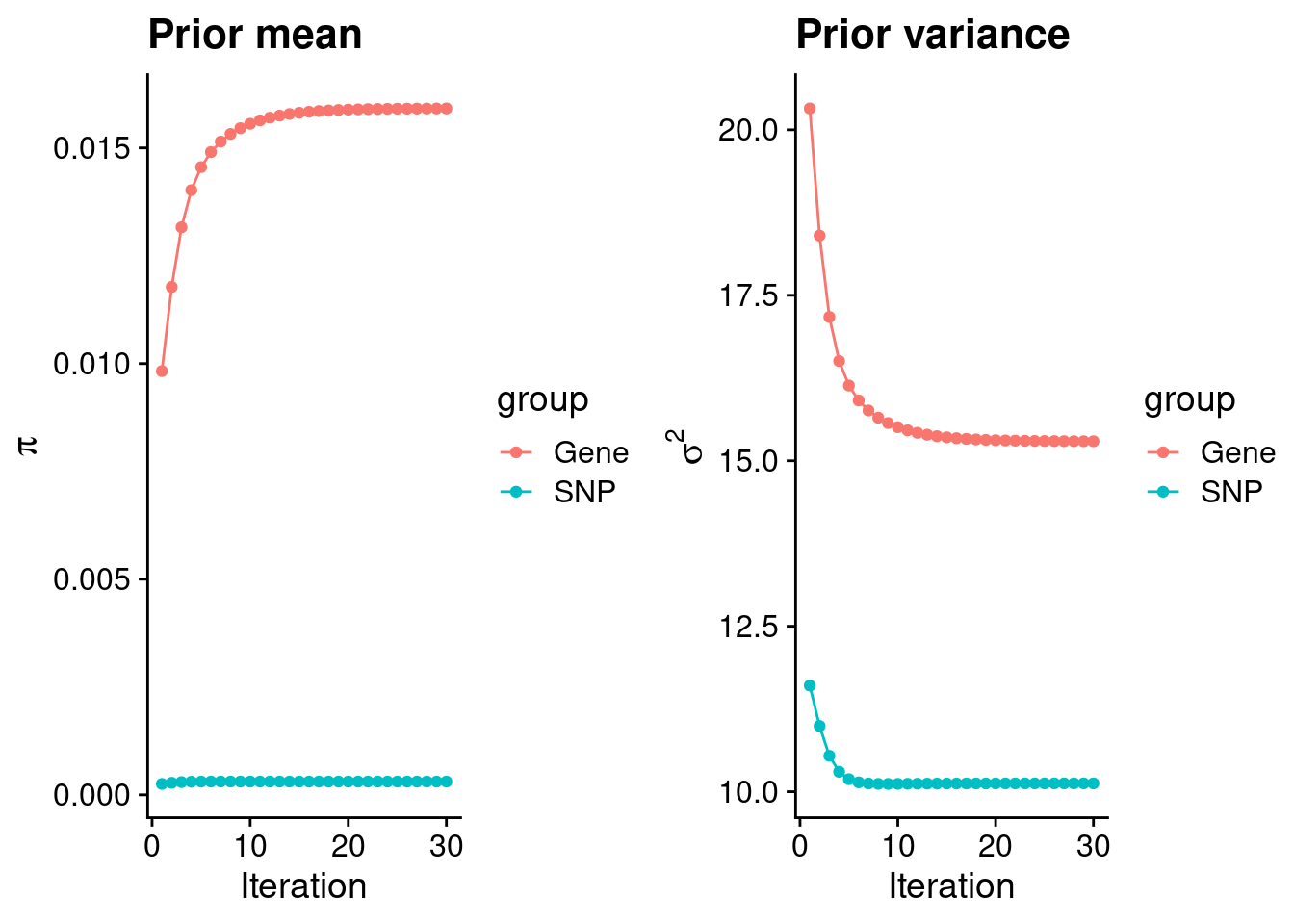
#estimated group prior
estimated_group_prior <- group_prior_rec[,ncol(group_prior_rec)]
names(estimated_group_prior) <- c("gene", "snp")
estimated_group_prior["snp"] <- estimated_group_prior["snp"]*thin #adjust parameter to account for thin argument
print(estimated_group_prior)
gene snp
0.0159161 0.0003071 #estimated group prior variance
estimated_group_prior_var <- group_prior_var_rec[,ncol(group_prior_var_rec)]
names(estimated_group_prior_var) <- c("gene", "snp")
print(estimated_group_prior_var) gene snp
15.29 10.13 #report sample size
print(sample_size)[1] 105318#report group size
group_size <- c(nrow(ctwas_gene_res), n_snps)
print(group_size)[1] 9567 6309950#estimated group PVE
estimated_group_pve <- estimated_group_prior_var*estimated_group_prior*group_size/sample_size #check PVE calculation
names(estimated_group_pve) <- c("gene", "snp")
print(estimated_group_pve) gene snp
0.02211 0.18629 #compare sum(PIP*mu2/sample_size) with above PVE calculation
c(sum(ctwas_gene_res$PVE),sum(ctwas_snp_res$PVE))[1] 0.06816 1.05969Genes with highest PIPs
           genename region_tag susie_pip    mu2       PVE      z num_eqtl
10843        ZNF823      19_10    0.9887  37.85 0.0003553  6.177        2
3993         SPECC1      17_16    0.9816  30.03 0.0002799  5.366        2
5324          FURIN      15_42    0.9769  47.90 0.0004443 -6.990        1
11997    AC012074.2       2_15    0.9585  22.81 0.0002076  4.653        2
13402 RP11-408A13.3       9_12    0.9399  23.43 0.0002091  4.536        1
13055 RP11-247A12.7       9_66    0.9372  23.41 0.0002083  4.683        1
5526          SYTL1       1_19    0.9100  21.63 0.0001869  4.307        2
10699         PCBP2      12_33    0.9062  26.83 0.0002308  5.065        1
2970          SF3B1      2_117    0.9027  50.93 0.0004365  7.265        1
1089           RRN3      16_15    0.8937  21.71 0.0001843 -4.264        2
6683           VPS8      3_113    0.8883  21.34 0.0001800 -4.258        1
11948     HIST1H2BN       6_21    0.8851 106.45 0.0008946 13.396        1
105           ELAC2      17_11    0.8803  22.00 0.0001839  4.811        2
10218       TMEM222       1_19    0.8801  21.61 0.0001806  4.303        1
3872           IRF3      19_35    0.8691  41.43 0.0003419 -6.461        1
11817     LINC00242      6_112    0.8632  21.69 0.0001778  4.288        2
5315          FANCI      15_41    0.8333  24.57 0.0001944 -4.481        1
706             GAL      11_38    0.8285  25.84 0.0002033 -4.946        2
307            VRK2       2_38    0.8260  38.46 0.0003016  4.977        1
1685       PPP1R16B      20_23    0.7927  60.76 0.0004573  7.738        1
Genes with largest effect sizes
       genename region_tag susie_pip    mu2       PVE        z num_eqtl
11174      APOM       6_26 2.279e-04 226.12 4.893e-07  11.5895        1
11169   ABHD16A       6_26 1.873e-04 223.25 3.970e-07  11.5262        1
11166      MSH5       6_26 1.656e-04 223.12 3.508e-07  11.5179        2
12252       C4A       6_26 4.277e-05 216.43 8.790e-08  11.3259        1
10534  HLA-DRB1       6_26 3.042e-05 178.62 5.159e-08   6.2222        1
11172    GPANK1       6_26 6.166e-05 172.29 1.009e-07  10.2672        1
11663 LINC01623       6_22 2.055e-02 156.89 3.062e-05 -12.9094        1
11142      RNF5       6_26 6.939e-05 154.88 1.020e-07  10.0454        1
11139    NOTCH4       6_26 1.102e-03 153.59 1.607e-06   8.4528        3
11948 HIST1H2BN       6_21 8.851e-01 106.45 8.946e-04  13.3956        1
11143    AGPAT1       6_26 3.964e-07 103.89 3.910e-10  -5.1903        1
10645  HLA-DQA1       6_26 4.324e-07 103.71 4.258e-10  -1.5380        1
11423    GTF2H4       6_25 3.997e-01 102.09 3.874e-04  11.1544        1
12073  HLA-DQA2       6_26 3.608e-07  92.84 3.180e-10   0.8591        1
9485   HLA-DQB1       6_26 3.438e-07  88.99 2.905e-10  -1.9898        1
11176      BAG6       6_26 3.345e-05  84.95 2.698e-08  -3.5825        1
9592  HIST1H2BC       6_20 3.365e-02  84.08 2.687e-05  -9.9088        1
4935      FLOT1       6_24 8.121e-02  83.84 6.465e-05 -10.9213        1
2696     TRIM38       6_20 2.313e-02  76.36 1.677e-05  -9.5948        2
11162    HSPA1A       6_26 2.791e-05  75.84 2.010e-08   8.0745        1
Genes with highest PVE
           genename region_tag susie_pip    mu2       PVE      z num_eqtl
11948     HIST1H2BN       6_21    0.8851 106.45 0.0008946 13.396        1
1685       PPP1R16B      20_23    0.7927  60.76 0.0004573  7.738        1
5324          FURIN      15_42    0.9769  47.90 0.0004443 -6.990        1
2970          SF3B1      2_117    0.9027  50.93 0.0004365  7.265        1
11423        GTF2H4       6_25    0.3997 102.09 0.0003874 11.154        1
10843        ZNF823      19_10    0.9887  37.85 0.0003553  6.177        2
3872           IRF3      19_35    0.8691  41.43 0.0003419 -6.461        1
10406       SLC38A3       3_35    0.7871  45.54 0.0003403 -1.402        1
2829           PCCB       3_84    0.7304  45.14 0.0003130 -6.724        1
307            VRK2       2_38    0.8260  38.46 0.0003016  4.977        1
3993         SPECC1      17_16    0.9816  30.03 0.0002799  5.366        2
2505            MDK      11_28    0.5826  48.64 0.0002690 -7.159        1
38             RBM6       3_35    0.5159  54.01 0.0002645  3.221        1
7669          LETM2       8_34    0.6763  38.57 0.0002476 -6.067        1
10797           NMB      15_39    0.7173  35.79 0.0002438  5.881        1
10699         PCBP2      12_33    0.9062  26.83 0.0002308  5.065        1
3041          ALMS1       2_48    0.7001  34.07 0.0002265 -5.898        1
7382          THOC7       3_43    0.5650  40.56 0.0002176 -6.249        1
13402 RP11-408A13.3       9_12    0.9399  23.43 0.0002091  4.536        1
13055 RP11-247A12.7       9_66    0.9372  23.41 0.0002083  4.683        1
Genes with largest z scores
genename region_tag susie_pip mu2 PVE z num_eqtl
11948 HIST1H2BN 6_21 8.851e-01 106.45 8.946e-04 13.396 1
11663 LINC01623 6_22 2.055e-02 156.89 3.062e-05 -12.909 1
11174 APOM 6_26 2.279e-04 226.12 4.893e-07 11.590 1
11169 ABHD16A 6_26 1.873e-04 223.25 3.970e-07 11.526 1
11166 MSH5 6_26 1.656e-04 223.12 3.508e-07 11.518 2
12252 C4A 6_26 4.277e-05 216.43 8.790e-08 11.326 1
11423 GTF2H4 6_25 3.997e-01 102.09 3.874e-04 11.154 1
4935 FLOT1 6_24 8.121e-02 83.84 6.465e-05 -10.921 1
11172 GPANK1 6_26 6.166e-05 172.29 1.009e-07 10.267 1
11142 RNF5 6_26 6.939e-05 154.88 1.020e-07 10.045 1
9592 HIST1H2BC 6_20 3.365e-02 84.08 2.687e-05 -9.909 1
10512 ZKSCAN3 6_22 2.276e-02 67.06 1.449e-05 9.707 2
2696 TRIM38 6_20 2.313e-02 76.36 1.677e-05 -9.595 2
10214 BTN3A2 6_20 2.116e-02 72.00 1.446e-05 9.294 2
11131 HLA-DMA 6_27 5.646e-02 68.13 3.652e-05 -8.590 2
11139 NOTCH4 6_26 1.102e-03 153.59 1.607e-06 8.453 3
11162 HSPA1A 6_26 2.791e-05 75.84 2.010e-08 8.075 1
11479 AS3MT 10_66 4.244e-01 45.06 1.816e-04 8.051 1
10360 ZSCAN23 6_22 7.931e-02 49.55 3.732e-05 -7.778 2
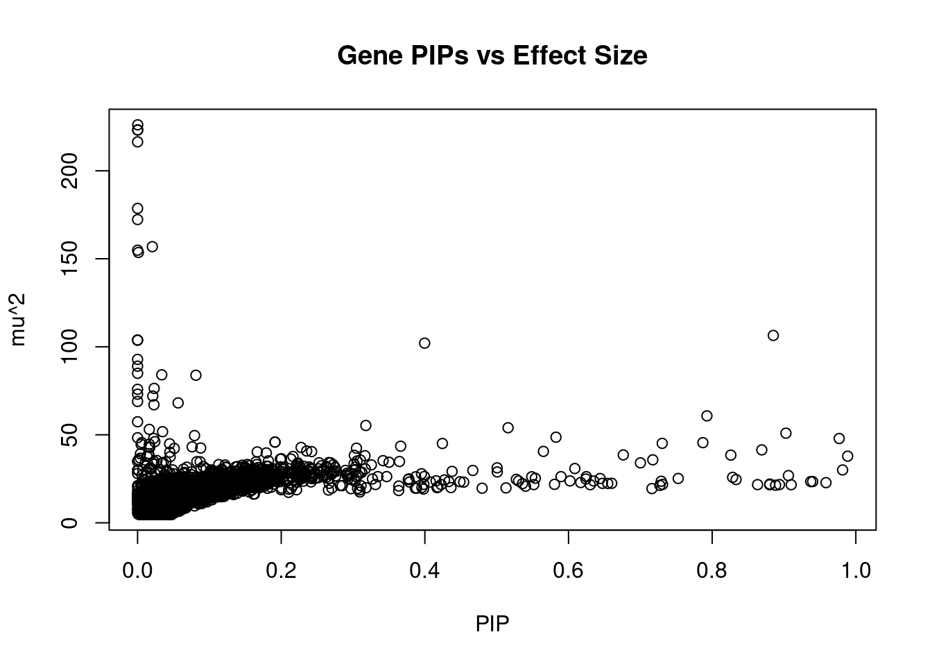
1685 PPP1R16B 20_23 7.927e-01 60.76 4.573e-04 7.738 1Comparing z scores and PIPs
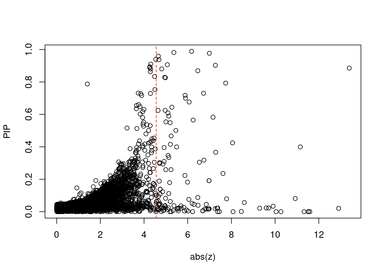
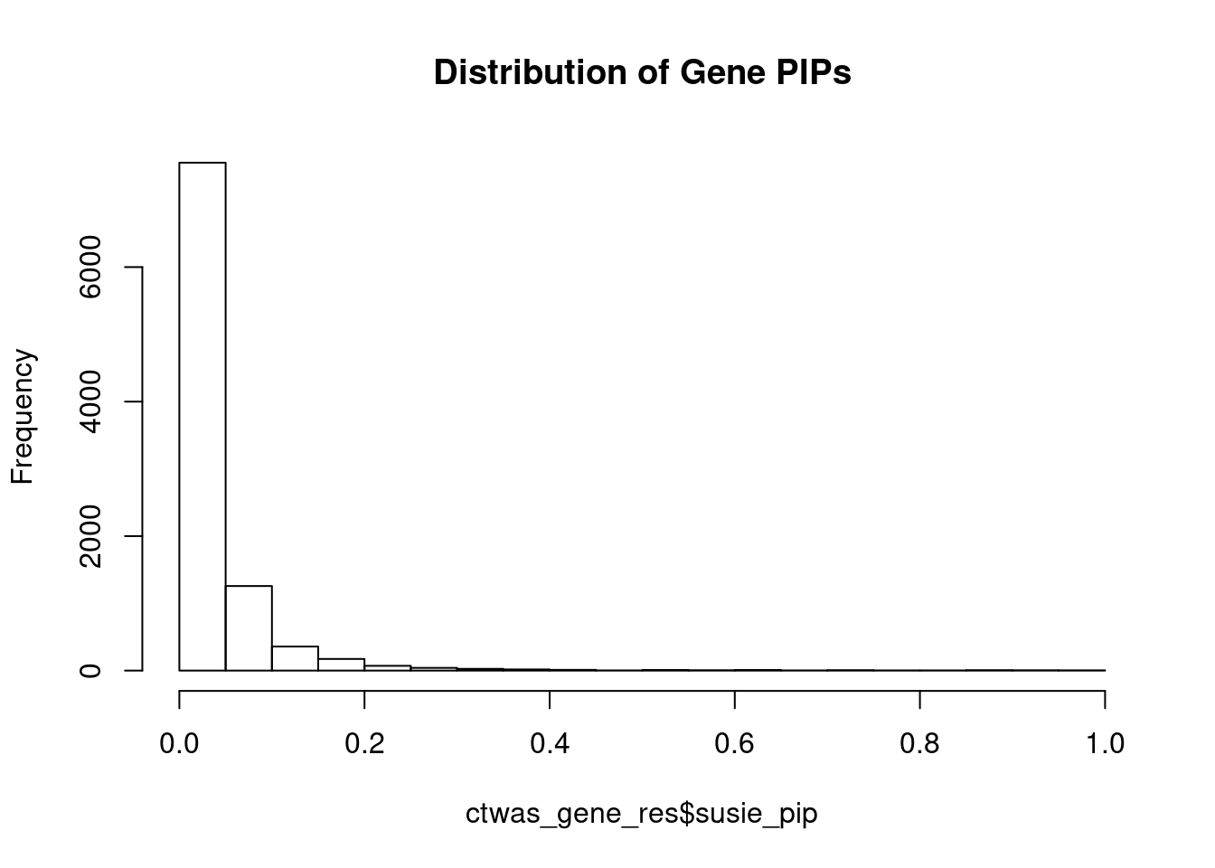
[1] 0.0138GO enrichment analysis for genes with PIP>0.5
#number of genes for gene set enrichment
length(genes)
[1] 56Uploading data to Enrichr... Done.
Querying GO_Biological_Process_2021... Done.
Querying GO_Cellular_Component_2021... Done.
Querying GO_Molecular_Function_2021... Done.
Parsing results... Done.
[1] "GO_Biological_Process_2021"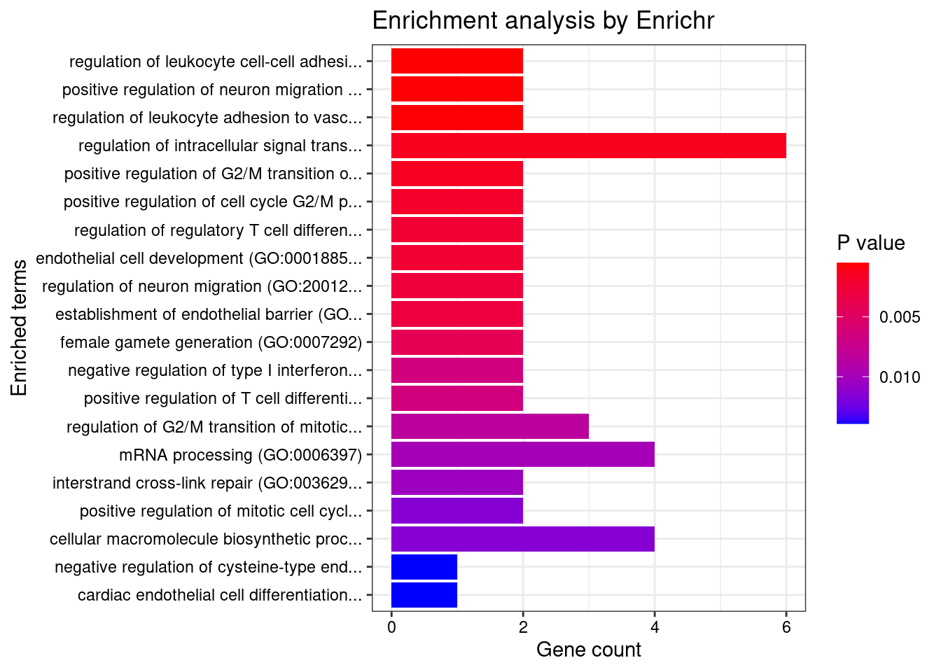
[1] Term             Overlap          Adjusted.P.value Genes
<0 rows> (or 0-length row.names)
[1] "GO_Cellular_Component_2021"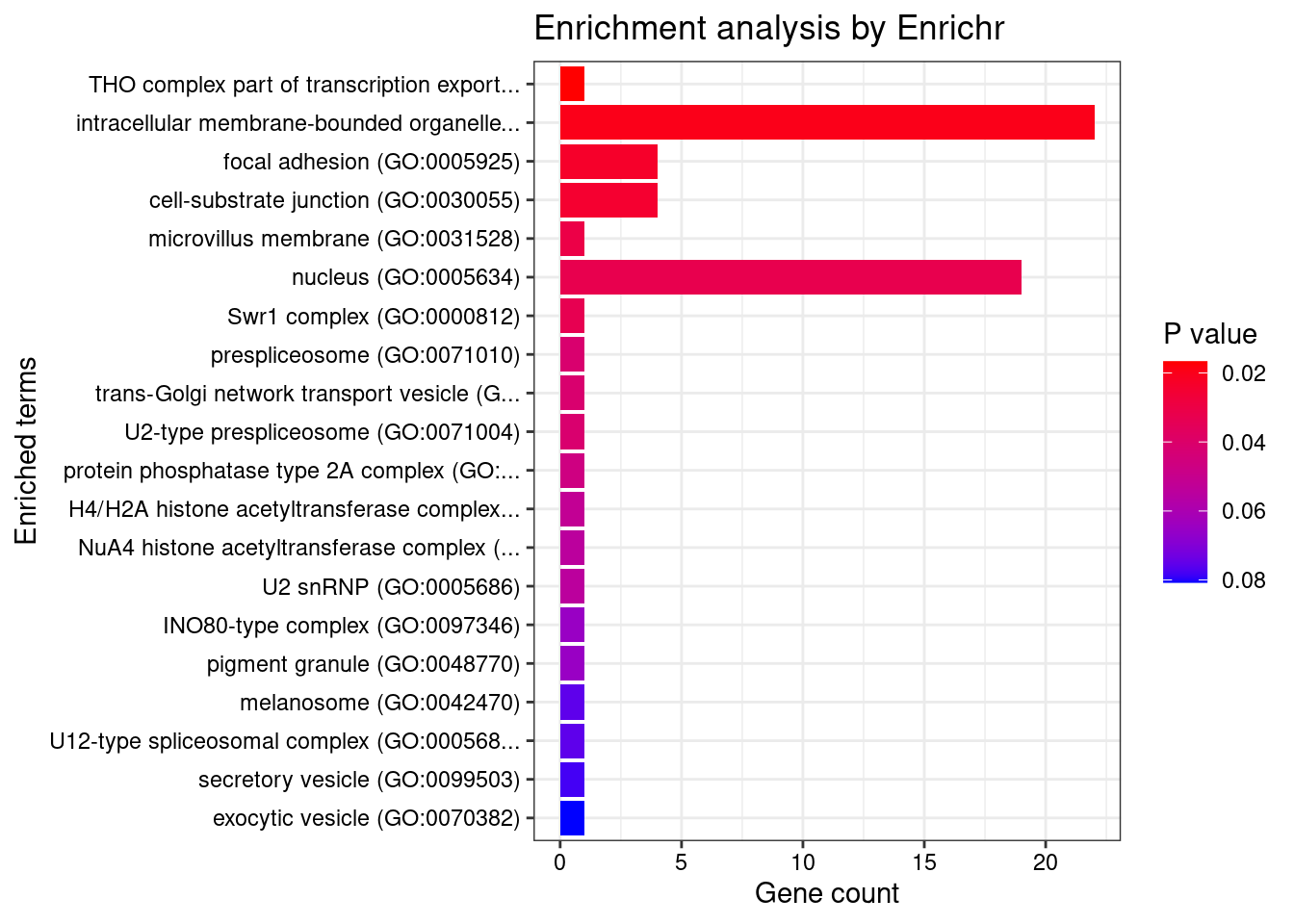
[1] Term             Overlap          Adjusted.P.value Genes
<0 rows> (or 0-length row.names)
[1] "GO_Molecular_Function_2021"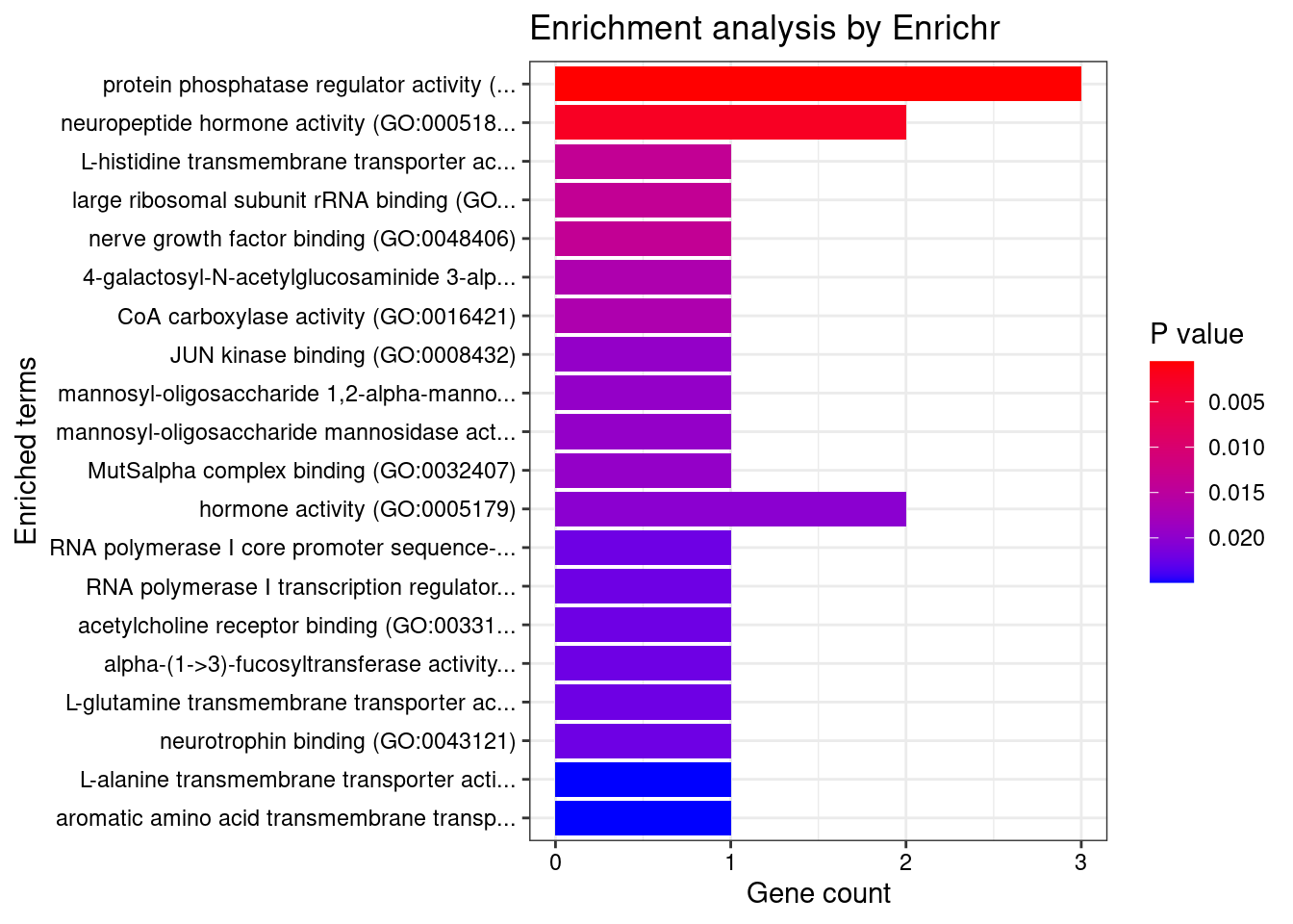
[1] Term             Overlap          Adjusted.P.value Genes
<0 rows> (or 0-length row.names)
DisGeNET enrichment analysis for genes with PIP>0.5
                                                                         Description
58                                                                  Alstrom Syndrome
105                                          FANCONI ANEMIA, COMPLEMENTATION GROUP I
107                                 HYPOTRICHOSIS-LYMPHEDEMA-TELANGIECTASIA SYNDROME
109                                                  Childhood-onset truncal obesity
115                MITOCHONDRIAL COMPLEX V (ATP SYNTHASE) DEFICIENCY, NUCLEAR TYPE 1
117                                                   PROSTATE CANCER, HEREDITARY, 2
119                                 COMBINED OXIDATIVE PHOSPHORYLATION DEFICIENCY 17
120                                                             OVARIAN DYSGENESIS 4
121 ENCEPHALOPATHY, ACUTE, INFECTION-INDUCED (HERPES-SPECIFIC), SUSCEPTIBILITY TO, 7
122                                              EPILEPSY, FAMILIAL TEMPORAL LOBE, 8
        FDR Ratio BgRatio
58  0.02273  1/21  1/9703
105 0.02273  1/21  1/9703
107 0.02273  1/21  1/9703
109 0.02273  1/21  1/9703
115 0.02273  1/21  1/9703
117 0.02273  1/21  1/9703
119 0.02273  1/21  1/9703
120 0.02273  1/21  1/9703
121 0.02273  1/21  1/9703
122 0.02273  1/21  1/9703
WebGestalt enrichment analysis for genes with PIP>0.5
Loading the functional categories...
Loading the ID list...
Loading the reference list...
Performing the enrichment analysis...
Warning in oraEnrichment(interestGeneList, referenceGeneList, geneSet, minNum =
minNum, : No significant gene set is identified based on FDR 0.05!NULLPIP Manhattan Plot
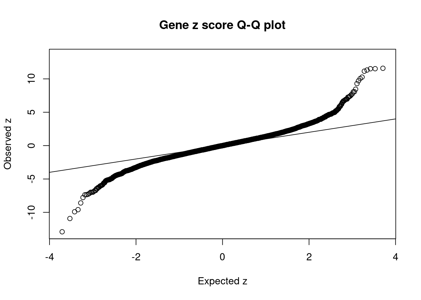
Warning: ggrepel: 4 unlabeled data points (too many overlaps). Consider
increasing max.overlaps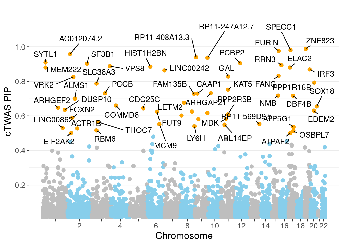
Sensitivity, specificity and precision for silver standard genes
#number of genes in known annotations
print(length(known_annotations))
[1] 130#number of genes in known annotations with imputed expression
print(sum(known_annotations %in% ctwas_gene_res$genename))[1] 57#significance threshold for TWAS
print(sig_thresh)[1] 4.555#number of ctwas genes
length(ctwas_genes)[1] 19#number of TWAS genes
length(twas_genes)[1] 132#show novel genes (ctwas genes with not in TWAS genes)
ctwas_gene_res[ctwas_gene_res$genename %in% novel_genes,report_cols] genename region_tag susie_pip mu2 PVE z num_eqtl
5526 SYTL1 1_19 0.9100 21.63 0.0001869 4.307 2
10218 TMEM222 1_19 0.8801 21.61 0.0001806 4.303 1
6683 VPS8 3_113 0.8883 21.34 0.0001800 -4.258 1
11817 LINC00242 6_112 0.8632 21.69 0.0001778 4.288 2
13402 RP11-408A13.3 9_12 0.9399 23.43 0.0002091 4.536 1
5315 FANCI 15_41 0.8333 24.57 0.0001944 -4.481 1
1089 RRN3 16_15 0.8937 21.71 0.0001843 -4.264 2#sensitivity / recall
print(sensitivity) ctwas TWAS
0.03846 0.10769 #specificity
print(specificity) ctwas TWAS
0.9985 0.9876 #precision / PPV
print(precision) ctwas TWAS
0.2632 0.1061 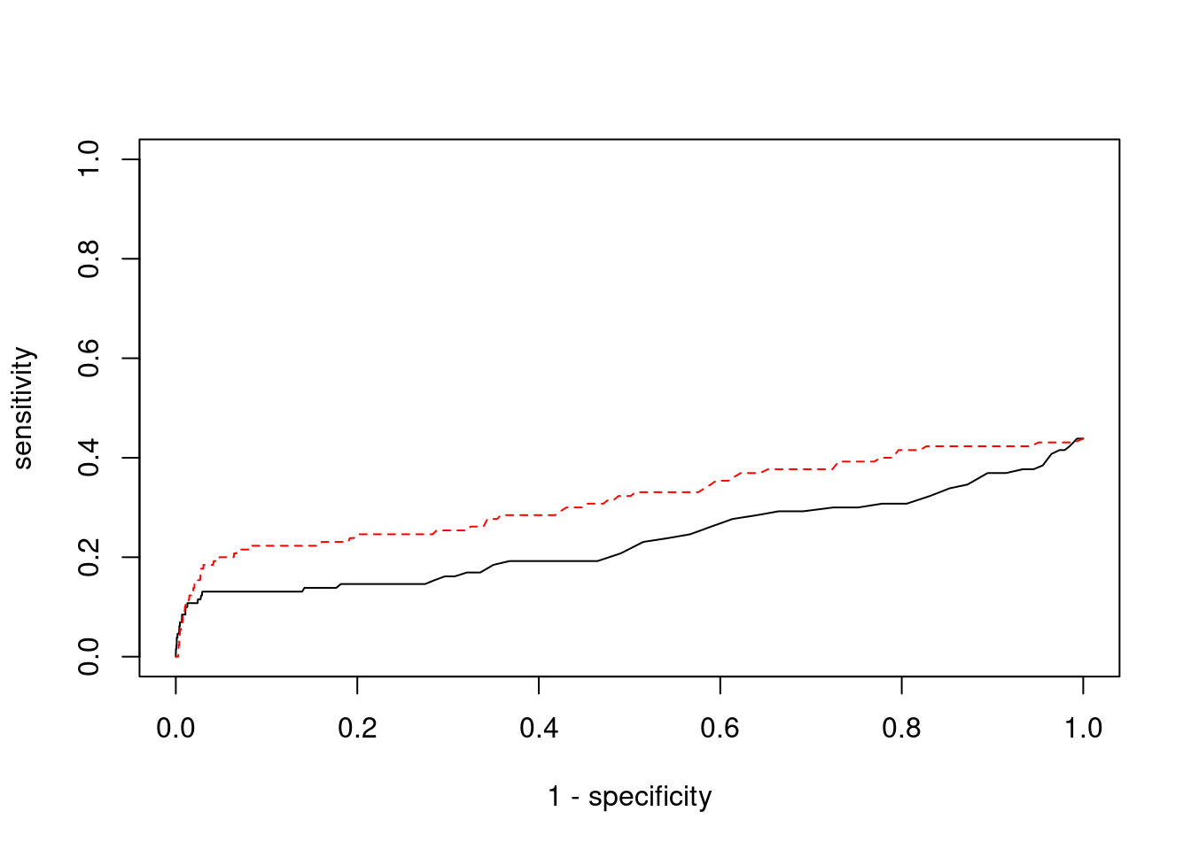
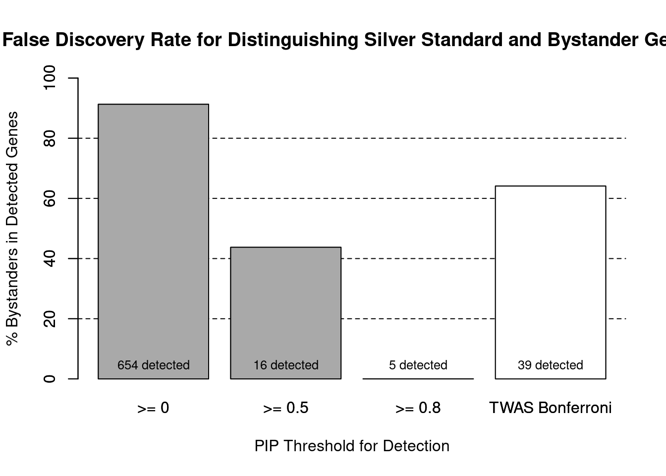
cTWAS is more precise than TWAS in distinguishing silver standard and bystander genes
#number of genes in known annotations (with imputed expression)
print(length(known_annotations))[1] 57#number of bystander genes (with imputed expression)
print(length(unrelated_genes))[1] 596#subset results to genes in known annotations or bystanders
ctwas_gene_res_subset <- ctwas_gene_res[ctwas_gene_res$genename %in% c(known_annotations, unrelated_genes),]
#assign ctwas and TWAS genes
ctwas_genes <- ctwas_gene_res_subset$genename[ctwas_gene_res_subset$susie_pip>0.8]
twas_genes <- ctwas_gene_res_subset$genename[abs(ctwas_gene_res_subset$z)>sig_thresh]
#significance threshold for TWAS
print(sig_thresh)
[1] 4.555#number of ctwas genes (in known annotations or bystanders)
length(ctwas_genes)[1] 5#number of TWAS genes (in known annotations or bystanders)
length(twas_genes)[1] 39#sensitivity / recall
sensitivity ctwas TWAS
0.08772 0.24561 #specificity / (1 - False Positive Rate)
specificity ctwas TWAS
1.0000 0.9581 #precision / PPV / (1 - False Discovery Rate)
precisionctwas TWAS
1.000 0.359 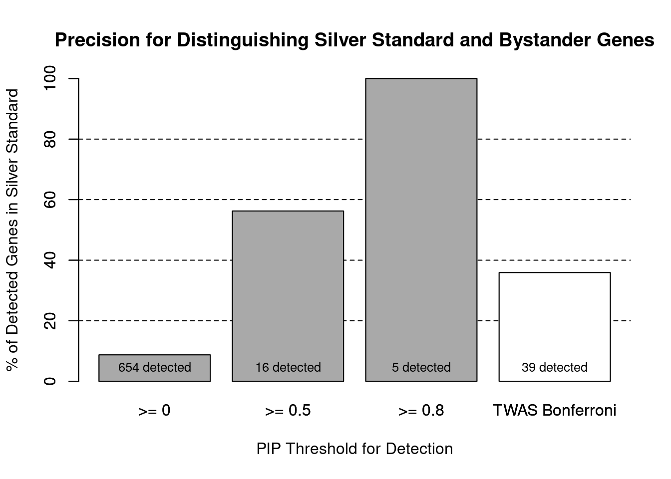
pip_range <- (0:1000)/1000
sensitivity <- rep(NA, length(pip_range))
specificity <- rep(NA, length(pip_range))

for (index in 1:length(pip_range)){
  pip <- pip_range[index]
  ctwas_genes <- ctwas_gene_res_subset$genename[ctwas_gene_res_subset$susie_pip>=pip]
  sensitivity[index] <- sum(ctwas_genes %in% known_annotations)/length(known_annotations)
  specificity[index] <- sum(!(unrelated_genes %in% ctwas_genes))/length(unrelated_genes)
}

plot(1-specificity, sensitivity, type="l", xlim=c(0,1), ylim=c(0,1), main="", xlab="1 - Specificity", ylab="Sensitivity")
title(expression("ROC Curve for cTWAS (black) and TWAS (" * phantom("red") * ")"))
title(expression(phantom("ROC Curve for cTWAS (black) and TWAS (") * "red" * phantom(")")), col.main="red")

sig_thresh_range <- seq(from=0, to=max(abs(ctwas_gene_res_subset$z)), length.out=length(pip_range))

for (index in 1:length(sig_thresh_range)){
  sig_thresh_plot <- sig_thresh_range[index]
  twas_genes <- ctwas_gene_res_subset$genename[abs(ctwas_gene_res_subset$z)>=sig_thresh_plot]
  sensitivity[index] <- sum(twas_genes %in% known_annotations)/length(known_annotations)
  specificity[index] <- sum(!(unrelated_genes %in% twas_genes))/length(unrelated_genes)
}

lines(1-specificity, sensitivity, xlim=c(0,1), ylim=c(0,1), col="red", lty=1)

abline(a=0,b=1,lty=3)

#add previously computed points from the analysis
ctwas_genes <- ctwas_gene_res_subset$genename[ctwas_gene_res_subset$susie_pip>0.8]
twas_genes <- ctwas_gene_res_subset$genename[abs(ctwas_gene_res_subset$z)>sig_thresh]

points(1-specificity_plot["ctwas"], sensitivity_plot["ctwas"], pch=21, bg="black")
points(1-specificity_plot["TWAS"], sensitivity_plot["TWAS"], pch=21, bg="red")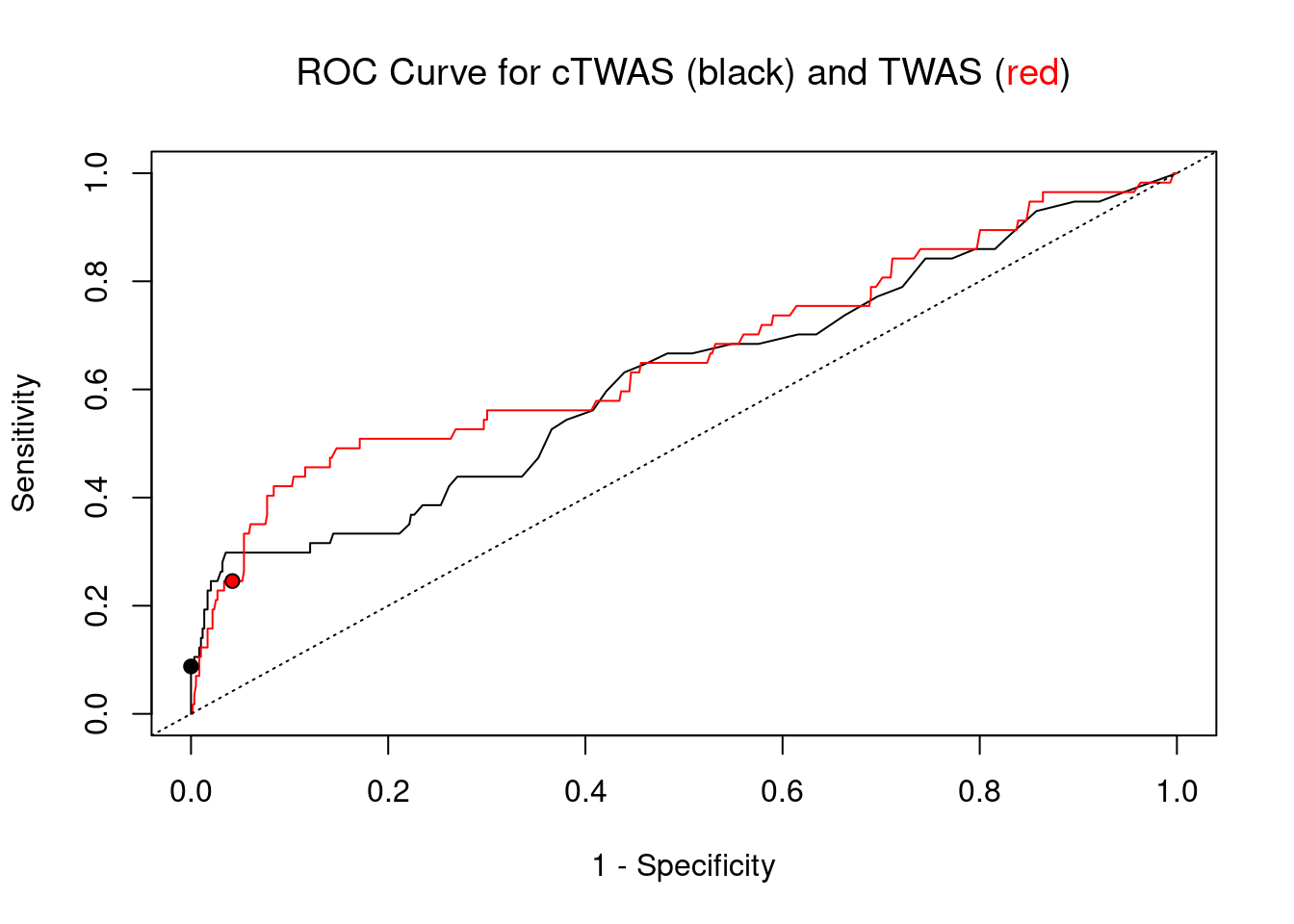
Undetected silver standard genes have low TWAS z-scores or stronger signal from nearby variants
#table of outcomes for silver standard genes
-sort(-table(silver_standard_case))
silver_standard_case
Not Imputed Insignificant z-score Nearby SNP(s)
73 43 9
Detected (PIP > 0.8)
5 #show inconclusive genes
silver_standard_case[silver_standard_case=="Inconclusive"]named character(0)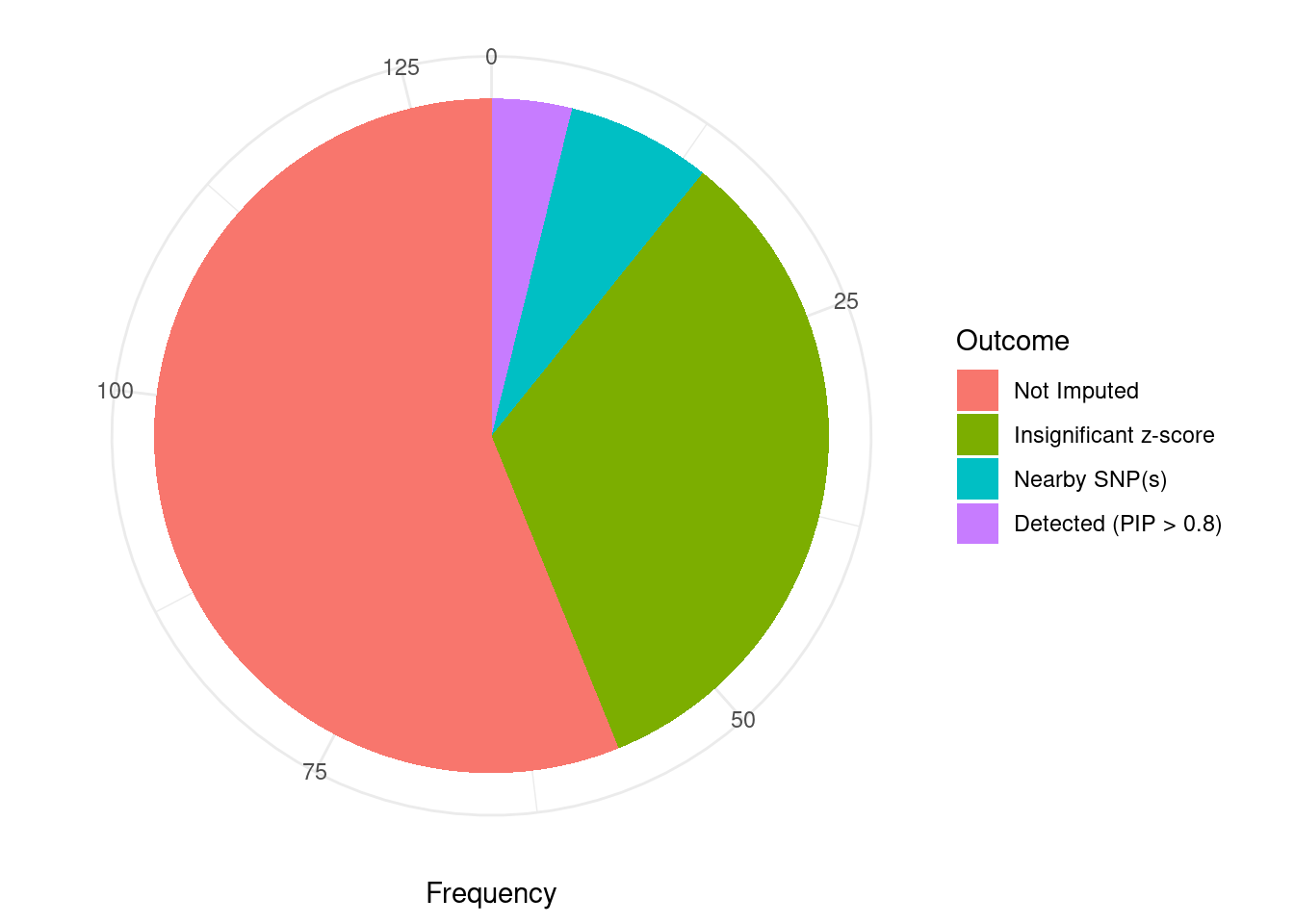
sessionInfo()R version 3.6.1 (2019-07-05)
Platform: x86_64-pc-linux-gnu (64-bit)
Running under: Scientific Linux 7.4 (Nitrogen)
Matrix products: default
BLAS/LAPACK: /software/openblas-0.2.19-el7-x86_64/lib/libopenblas_haswellp-r0.2.19.so
locale:
[1] LC_CTYPE=en_US.UTF-8 LC_NUMERIC=C
[3] LC_TIME=en_US.UTF-8 LC_COLLATE=en_US.UTF-8
[5] LC_MONETARY=en_US.UTF-8 LC_MESSAGES=en_US.UTF-8
[7] LC_PAPER=en_US.UTF-8 LC_NAME=C
[9] LC_ADDRESS=C LC_TELEPHONE=C
[11] LC_MEASUREMENT=en_US.UTF-8 LC_IDENTIFICATION=C
attached base packages:
[1] parallel stats4 stats graphics grDevices utils datasets
[8] methods base
other attached packages:
[1] GenomicRanges_1.36.1 GenomeInfoDb_1.20.0 IRanges_2.18.1
[4] S4Vectors_0.22.1 BiocGenerics_0.30.0 biomaRt_2.40.1
[7] readxl_1.3.1 forcats_0.5.1 stringr_1.4.0
[10] dplyr_1.0.7 purrr_0.3.4 readr_2.1.1
[13] tidyr_1.1.4 tidyverse_1.3.1 tibble_3.1.6
[16] WebGestaltR_0.4.4 disgenet2r_0.99.2 enrichR_3.0
[19] cowplot_1.1.1 ggplot2_3.3.5 workflowr_1.7.0
loaded via a namespace (and not attached):
[1] ggbeeswarm_0.6.0 colorspace_2.0-2 rjson_0.2.20
[4] ellipsis_0.3.2 rprojroot_2.0.2 XVector_0.24.0
[7] fs_1.5.2 rstudioapi_0.13 farver_2.1.0
[10] ggrepel_0.9.1 bit64_4.0.5 AnnotationDbi_1.46.0
[13] fansi_1.0.2 lubridate_1.8.0 xml2_1.3.3
[16] codetools_0.2-16 doParallel_1.0.17 cachem_1.0.6
[19] knitr_1.36 jsonlite_1.7.2 apcluster_1.4.8
[22] Cairo_1.5-12.2 broom_0.7.10 dbplyr_2.1.1
[25] compiler_3.6.1 httr_1.4.2 backports_1.4.1
[28] assertthat_0.2.1 Matrix_1.2-18 fastmap_1.1.0
[31] cli_3.1.0 later_0.8.0 prettyunits_1.1.1
[34] htmltools_0.5.2 tools_3.6.1 igraph_1.2.10
[37] GenomeInfoDbData_1.2.1 gtable_0.3.0 glue_1.6.2
[40] reshape2_1.4.4 doRNG_1.8.2 Rcpp_1.0.8
[43] Biobase_2.44.0 cellranger_1.1.0 jquerylib_0.1.4
[46] vctrs_0.3.8 svglite_1.2.2 iterators_1.0.14
[49] xfun_0.29 ps_1.6.0 rvest_1.0.2
[52] lifecycle_1.0.1 rngtools_1.5.2 XML_3.99-0.3
[55] zlibbioc_1.30.0 getPass_0.2-2 scales_1.1.1
[58] vroom_1.5.7 hms_1.1.1 promises_1.0.1
[61] yaml_2.2.1 curl_4.3.2 memoise_2.0.1
[64] ggrastr_1.0.1 gdtools_0.1.9 stringi_1.7.6
[67] RSQLite_2.2.8 highr_0.9 foreach_1.5.2
[70] rlang_1.0.1 pkgconfig_2.0.3 bitops_1.0-7
[73] evaluate_0.14 lattice_0.20-38 labeling_0.4.2
[76] bit_4.0.4 processx_3.5.2 tidyselect_1.1.1
[79] plyr_1.8.6 magrittr_2.0.2 R6_2.5.1
[82] generics_0.1.1 DBI_1.1.2 pillar_1.6.4
[85] haven_2.4.3 whisker_0.3-2 withr_2.4.3
[88] RCurl_1.98-1.5 modelr_0.1.8 crayon_1.5.0
[91] utf8_1.2.2 tzdb_0.2.0 rmarkdown_2.11
[94] progress_1.2.2 grid_3.6.1 data.table_1.14.2
[97] blob_1.2.2 callr_3.7.0 git2r_0.26.1
[100] reprex_2.0.1 digest_0.6.29 httpuv_1.5.1
[103] munsell_0.5.0 beeswarm_0.2.3 vipor_0.4.5