SCZ - Annotation Analysis
sheng Qian
2022-4-11
Last updated: 2022-04-18
Checks: 5 2
Knit directory: cTWAS_analysis/
This reproducible R Markdown analysis was created with workflowr (version 1.7.0). The Checks tab describes the reproducibility checks that were applied when the results were created. The Past versions tab lists the development history.
The R Markdown file has unstaged changes. To know which version of the R Markdown file created these results, you’ll want to first commit it to the Git repo. If you’re still working on the analysis, you can ignore this warning. When you’re finished, you can run wflow_publish to commit the R Markdown file and build the HTML.
Great job! The global environment was empty. Objects defined in the global environment can affect the analysis in your R Markdown file in unknown ways. For reproduciblity it’s best to always run the code in an empty environment.
The command set.seed(20211220) was run prior to running the code in the R Markdown file. Setting a seed ensures that any results that rely on randomness, e.g. subsampling or permutations, are reproducible.
Great job! Recording the operating system, R version, and package versions is critical for reproducibility.
Nice! There were no cached chunks for this analysis, so you can be confident that you successfully produced the results during this run.
Using absolute paths to the files within your workflowr project makes it difficult for you and others to run your code on a different machine. Change the absolute path(s) below to the suggested relative path(s) to make your code more reproducible.
| absolute | relative |
|---|---|
| /project2/xinhe/shengqian/cTWAS/cTWAS_analysis/data/SCZ_2014_EUR/ | data/SCZ_2014_EUR |
Great! You are using Git for version control. Tracking code development and connecting the code version to the results is critical for reproducibility.
The results in this page were generated with repository version 0552ba2. See the Past versions tab to see a history of the changes made to the R Markdown and HTML files.
Note that you need to be careful to ensure that all relevant files for the analysis have been committed to Git prior to generating the results (you can use wflow_publish or wflow_git_commit). workflowr only checks the R Markdown file, but you know if there are other scripts or data files that it depends on. Below is the status of the Git repository when the results were generated:
Ignored files:
    Ignored:    .ipynb_checkpoints/
    Ignored:    data/AF/

Untracked files:
    Untracked:  Rplot.png
    Untracked:  analysis/.ipynb_checkpoints/
    Untracked:  code/.ipynb_checkpoints/
    Untracked:  code/AF_out/
    Untracked:  code/Autism_out/
    Untracked:  code/BMI_S_out/
    Untracked:  code/BMI_out/
    Untracked:  code/Glucose_out/
    Untracked:  code/LDL_S_out/
    Untracked:  code/SCZ_2014_EUR_out/
    Untracked:  code/SCZ_2018_out/
    Untracked:  code/SCZ_2020_Single_out/
    Untracked:  code/SCZ_2020_out/
    Untracked:  code/SCZ_S_out/
    Untracked:  code/SCZ_out/
    Untracked:  code/T2D_out/
    Untracked:  code/ctwas_config.R
    Untracked:  code/mapping.R
    Untracked:  code/out/
    Untracked:  code/process_scz_2018_snps.R
    Untracked:  code/run_AF_analysis.sbatch
    Untracked:  code/run_AF_analysis.sh
    Untracked:  code/run_AF_ctwas_rss_LDR.R
    Untracked:  code/run_Autism_analysis.sbatch
    Untracked:  code/run_Autism_analysis.sh
    Untracked:  code/run_Autism_ctwas_rss_LDR.R
    Untracked:  code/run_BMI_analysis.sbatch
    Untracked:  code/run_BMI_analysis.sh
    Untracked:  code/run_BMI_analysis_S.sbatch
    Untracked:  code/run_BMI_analysis_S.sh
    Untracked:  code/run_BMI_ctwas_rss_LDR.R
    Untracked:  code/run_BMI_ctwas_rss_LDR_S.R
    Untracked:  code/run_Glucose_analysis.sbatch
    Untracked:  code/run_Glucose_analysis.sh
    Untracked:  code/run_Glucose_ctwas_rss_LDR.R
    Untracked:  code/run_LDL_analysis_S.sbatch
    Untracked:  code/run_LDL_analysis_S.sh
    Untracked:  code/run_LDL_ctwas_rss_LDR_S.R
    Untracked:  code/run_SCZ_2014_EUR_analysis.sbatch
    Untracked:  code/run_SCZ_2014_EUR_analysis.sh
    Untracked:  code/run_SCZ_2014_EUR_ctwas_rss_LDR.R
    Untracked:  code/run_SCZ_2018_analysis.sbatch
    Untracked:  code/run_SCZ_2018_analysis.sh
    Untracked:  code/run_SCZ_2018_ctwas_rss_LDR.R
    Untracked:  code/run_SCZ_2020_Single_analysis.sbatch
    Untracked:  code/run_SCZ_2020_Single_analysis.sh
    Untracked:  code/run_SCZ_2020_Single_ctwas_rss_LDR.R
    Untracked:  code/run_SCZ_2020_analysis.sbatch
    Untracked:  code/run_SCZ_2020_analysis.sh
    Untracked:  code/run_SCZ_2020_ctwas_rss_LDR.R
    Untracked:  code/run_SCZ_analysis.sbatch
    Untracked:  code/run_SCZ_analysis.sh
    Untracked:  code/run_SCZ_analysis_S.sbatch
    Untracked:  code/run_SCZ_analysis_S.sh
    Untracked:  code/run_SCZ_ctwas_rss_LDR.R
    Untracked:  code/run_SCZ_ctwas_rss_LDR_S.R
    Untracked:  code/run_T2D_analysis.sbatch
    Untracked:  code/run_T2D_analysis.sh
    Untracked:  code/run_T2D_ctwas_rss_LDR.R
    Untracked:  code/wflow_build.R
    Untracked:  code/wflow_build.sbatch
    Untracked:  data/.ipynb_checkpoints/
    Untracked:  data/BMI/
    Untracked:  data/PGC3_SCZ_wave3_public.v2.tsv
    Untracked:  data/SCZ/
    Untracked:  data/SCZ_2014_EUR/
    Untracked:  data/SCZ_2018/
    Untracked:  data/SCZ_2020/
    Untracked:  data/SCZ_2020_Single/
    Untracked:  data/SCZ_S/
    Untracked:  data/Supplementary Table 15 - MAGMA.xlsx
    Untracked:  data/Supplementary Table 20 - Prioritised Genes.xlsx
    Untracked:  data/T2D/
    Untracked:  data/UKBB/
    Untracked:  data/UKBB_SNPs_Info.text
    Untracked:  data/gene_OMIM.txt
    Untracked:  data/gene_pip_0.8.txt
    Untracked:  data/mashr_Heart_Atrial_Appendage.db
    Untracked:  data/mashr_sqtl/
    Untracked:  data/scz_2018.RDS
    Untracked:  data/summary_known_genes_annotations.xlsx
    Untracked:  data/untitled.txt
    Untracked:  top_genes_32.txt
    Untracked:  top_genes_37.txt
    Untracked:  top_genes_43.txt
    Untracked:  top_genes_81.txt

Unstaged changes:
    Modified:   analysis/SCZ_Annotation_Analysis.Rmd
Note that any generated files, e.g. HTML, png, CSS, etc., are not included in this status report because it is ok for generated content to have uncommitted changes.
These are the previous versions of the repository in which changes were made to the R Markdown (analysis/SCZ_Annotation_Analysis.Rmd) and HTML (docs/SCZ_Annotation_Analysis.html) files. If you’ve configured a remote Git repository (see ?wflow_git_remote), click on the hyperlinks in the table below to view the files as they were in that past version.
| File | Version | Author | Date | Message |
|---|---|---|---|---|
| Rmd | 0552ba2 | sq-96 | 2022-04-18 | update |
| html | 0552ba2 | sq-96 | 2022-04-18 | update |
| Rmd | 9ddc9c4 | sq-96 | 2022-04-18 | update |
| Rmd | f6e7062 | sq-96 | 2022-04-17 | update |
brain_tissue <- list.files("/project2/xinhe/shengqian/cTWAS/cTWAS_analysis/data/SCZ_2014_EUR/")
top_genes <- c()
all_genes <- c()
for(i in brain_tissue){
  df <- readRDS(paste0("/project2/xinhe/shengqian/cTWAS/cTWAS_analysis/data/SCZ_2014_EUR/",i,"/SCZ_",i,"_ctwas_gene_res.RDS"))
  all_genes <- c(all_genes,df$genename)
  df <- df[df$susie_pip>=0.5,]
  top_genes <- c(top_genes,df$genename)
}
top_genes <- unique(top_genes)
all_genes <- unique(all_genes)
set.seed(2022)
random_genes <- sample(all_genes,1000)
library(readxl)
Supplementary_Table_15_MAGMA <- read_excel("data/Supplementary Table 15 - MAGMA.xlsx",
sheet = "Gene Lists")
summary_known_genes_annotations <- read_excel("data/summary_known_genes_annotations.xlsx",
sheet = "SCZ")
SCHEMA_genes <- Supplementary_Table_15_MAGMA$`SCHEMA (p<0.001)`
SCHEMA_genes <- SCHEMA_genes[!is.na(SCHEMA_genes)]
ASD_genes <- Supplementary_Table_15_MAGMA$`ASD (Satterstrom et al. 2019)`
ASD_genes <- ASD_genes[!is.na(ASD_genes)]
DDD_genes <- Supplementary_Table_15_MAGMA$`DDD (Kaplanis et al. 2019)`
DDD_genes <- DDD_genes[!is.na(DDD_genes)]
PGC3_genes <- summary_known_genes_annotations$`Gene Symbol`
PGC3_genes <- PGC3_genes[!is.na(PGC3_genes)]Supplementary_Table_20_Prioritised_Genes <- read_excel("data/Supplementary Table 20 - Prioritised Genes.xlsx",
sheet = "ST20 all criteria")
SMR_genes <- Supplementary_Table_20_Prioritised_Genes[,c("Symbol.ID","SMRmap","SMRsingleGene","HI.C.SMR")]
SMR_genes["index"] <- (SMR_genes$SMRmap==1) | (SMR_genes$SMRsingleGene==1) | (SMR_genes$HI.C.SMR==1)
SMR_genes <- SMR_genes[SMR_genes$index==1,]$Symbol.IDsum(top_genes %in% SCHEMA_genes)[1] 2sum(top_genes %in% ASD_genes)[1] 1sum(top_genes %in% DDD_genes)[1] 5sum(top_genes %in% PGC3_genes)[1] 9sum(top_genes %in% setdiff(PGC3_genes,SMR_genes))[1] 1sum(random_genes %in% SCHEMA_genes)[1] 3sum(random_genes %in% ASD_genes)[1] 7sum(random_genes %in% DDD_genes)[1] 14sum(random_genes %in% PGC3_genes)[1] 6sum(random_genes %in% setdiff(PGC3_genes,SMR_genes))[1] 4fisher.test(matrix(c(sum(top_genes %in% SCHEMA_genes),length(top_genes)-sum(top_genes %in% SCHEMA_genes),sum(random_genes %in% SCHEMA_genes),1000-sum(random_genes %in% SCHEMA_genes)),ncol=2))
    Fisher's Exact Test for Count Data

data:
p-value = 0.1413
alternative hypothesis: true odds ratio is not equal to 1
95 percent confidence interval:
  0.350347 37.179757
sample estimates:
odds ratio
  4.225739
fisher.test(matrix(c(sum(top_genes %in% ASD_genes),length(top_genes)-sum(top_genes %in% ASD_genes),sum(random_genes %in% ASD_genes),1000-sum(random_genes %in% ASD_genes)),ncol=2))
    Fisher's Exact Test for Count Data

data:
p-value = 1
alternative hypothesis: true odds ratio is not equal to 1
95 percent confidence interval:
 0.01979746 7.06655191
sample estimates:
odds ratio
  0.897886
fisher.test(matrix(c(sum(top_genes %in% DDD_genes),length(top_genes)-sum(top_genes %in% DDD_genes),sum(random_genes %in% DDD_genes),1000-sum(random_genes %in% DDD_genes)),ncol=2))
    Fisher's Exact Test for Count Data

data:
p-value = 0.1657
alternative hypothesis: true odds ratio is not equal to 1
95 percent confidence interval:
 0.6348484 6.8334851
sample estimates:
odds ratio
  2.284503
fisher.test(matrix(c(sum(top_genes %in% PGC3_genes),length(top_genes)-sum(top_genes %in% PGC3_genes),sum(random_genes %in% PGC3_genes),1000-sum(random_genes %in% PGC3_genes)),ncol=2))
    Fisher's Exact Test for Count Data

data:
p-value = 3.34e-05
alternative hypothesis: true odds ratio is not equal to 1
95 percent confidence interval:
  3.09800 34.34657
sample estimates:
odds ratio
  9.904212
fisher.test(matrix(c(sum(top_genes %in% setdiff(PGC3_genes,SMR_genes)),length(top_genes)-sum(top_genes %in% setdiff(PGC3_genes,SMR_genes)),sum(random_genes %in% setdiff(PGC3_genes,SMR_genes)),1000-sum(random_genes %in% setdiff(PGC3_genes,SMR_genes))),ncol=2))
    Fisher's Exact Test for Count Data

data:
p-value = 0.5225
alternative hypothesis: true odds ratio is not equal to 1
95 percent confidence interval:
  0.03180166 16.04506772
sample estimates:
odds ratio
1.575219 library(enrichR)Welcome to enrichR
Checking connection ... Enrichr ... Connection is Live!
FlyEnrichr ... Connection is available!
WormEnrichr ... Connection is available!
YeastEnrichr ... Connection is available!
FishEnrichr ... Connection is available!dbs <- c("GO_Biological_Process_2021", "GO_Cellular_Component_2021", "GO_Molecular_Function_2021")
if (length(top_genes)>0){
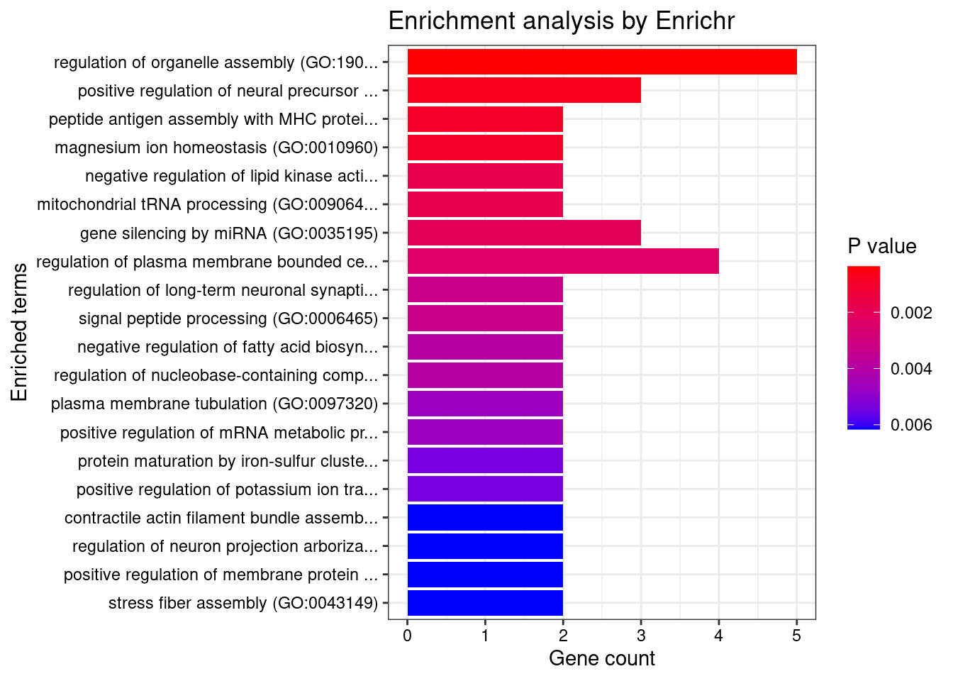
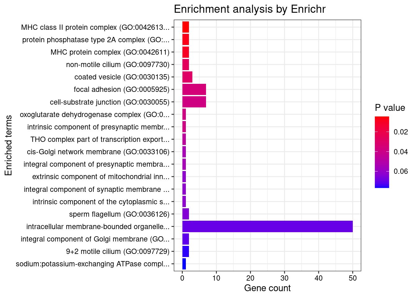
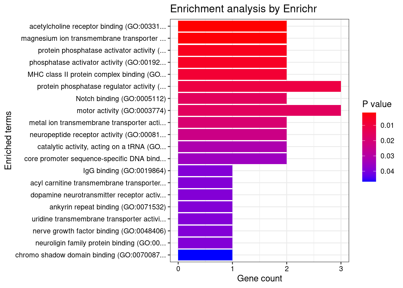
GO_enrichment <- enrichr(top_genes, dbs)
for (db in dbs){
print(db)
df <- GO_enrichment[[db]]
print(plotEnrich(GO_enrichment[[db]]))
df <- df[df$Adjusted.P.value<0.05,c("Term", "Overlap", "Adjusted.P.value", "Genes")]
print(df)
}
}Uploading data to Enrichr... Done.
Querying GO_Biological_Process_2021... Done.
Querying GO_Cellular_Component_2021... Done.
Querying GO_Molecular_Function_2021... Done.
Parsing results... Done.
[1] "GO_Biological_Process_2021"
| Version | Author | Date |
|---|---|---|
| 0552ba2 | sq-96 | 2022-04-18 |
[1] Term             Overlap          Adjusted.P.value Genes
<0 rows> (or 0-length row.names)
[1] "GO_Cellular_Component_2021"
| Version | Author | Date |
|---|---|---|
| 0552ba2 | sq-96 | 2022-04-18 |
[1] Term             Overlap          Adjusted.P.value Genes
<0 rows> (or 0-length row.names)
[1] "GO_Molecular_Function_2021"
| Version | Author | Date |
|---|---|---|
| 0552ba2 | sq-96 | 2022-04-18 |
[1] Term             Overlap          Adjusted.P.value Genes
<0 rows> (or 0-length row.names)
Description FDR Ratio BgRatio
84 Measles 0.04999924 1/65 1/9703
106 Schizophrenia 0.04999924 13/65 883/9703
108 Spasmophilia 0.04999924 1/65 1/9703
116 Tachycardia 0.04999924 2/65 18/9703
117 Tetany 0.04999924 1/65 1/9703
123 Tachyarrhythmia 0.04999924 2/65 18/9703
179 Alstrom Syndrome 0.04999924 1/65 1/9703
180 Tetany, Neonatal 0.04999924 1/65 1/9703
210 Renal dysplasia and retinal aplasia (disorder) 0.04999924 2/65 12/9703
277 Bardet-Biedl Syndrome 0.04999924 2/65 13/9703
sessionInfo()R version 3.6.1 (2019-07-05)
Platform: x86_64-pc-linux-gnu (64-bit)
Running under: Scientific Linux 7.4 (Nitrogen)
Matrix products: default
BLAS/LAPACK: /software/openblas-0.2.19-el7-x86_64/lib/libopenblas_haswellp-r0.2.19.so
locale:
[1] LC_CTYPE=en_US.UTF-8 LC_NUMERIC=C
[3] LC_TIME=en_US.UTF-8 LC_COLLATE=en_US.UTF-8
[5] LC_MONETARY=en_US.UTF-8 LC_MESSAGES=en_US.UTF-8
[7] LC_PAPER=en_US.UTF-8 LC_NAME=C
[9] LC_ADDRESS=C LC_TELEPHONE=C
[11] LC_MEASUREMENT=en_US.UTF-8 LC_IDENTIFICATION=C
attached base packages:
[1] stats graphics grDevices utils datasets methods base
other attached packages:
[1] disgenet2r_0.99.2 enrichR_3.0 readxl_1.3.1 workflowr_1.7.0
loaded via a namespace (and not attached):
[1] tidyselect_1.1.1 xfun_0.29 reshape2_1.4.4 purrr_0.3.4
[5] colorspace_2.0-2 vctrs_0.3.8 generics_0.1.1 htmltools_0.5.2
[9] yaml_2.2.1 utf8_1.2.2 rlang_1.0.1 later_0.8.0
[13] pillar_1.6.4 jquerylib_0.1.4 glue_1.6.2 DBI_1.1.2
[17] plyr_1.8.6 lifecycle_1.0.1 stringr_1.4.0 munsell_0.5.0
[21] gtable_0.3.0 cellranger_1.1.0 evaluate_0.14 labeling_0.4.2
[25] knitr_1.36 callr_3.7.0 fastmap_1.1.0 httpuv_1.5.1
[29] ps_1.6.0 curl_4.3.2 fansi_1.0.2 highr_0.9
[33] Rcpp_1.0.8 promises_1.0.1 scales_1.1.1 jsonlite_1.7.2
[37] farver_2.1.0 fs_1.5.2 rjson_0.2.20 ggplot2_3.3.5
[41] digest_0.6.29 stringi_1.7.6 processx_3.5.2 dplyr_1.0.7
[45] getPass_0.2-2 rprojroot_2.0.2 grid_3.6.1 cli_3.1.0
[49] tools_3.6.1 magrittr_2.0.2 tibble_3.1.6 crayon_1.5.0
[53] whisker_0.3-2 pkgconfig_2.0.3 ellipsis_0.3.2 assertthat_0.2.1
[57] rmarkdown_2.11 httr_1.4.2 rstudioapi_0.13 R6_2.5.1
[61] git2r_0.26.1 compiler_3.6.1