BMI - Brain Caudate basal ganglia
sheng Qian
2021-2-6
Last updated: 2022-02-13
Checks: 6 1
Knit directory: cTWAS_analysis/
This reproducible R Markdown analysis was created with workflowr (version 1.6.2). The Checks tab describes the reproducibility checks that were applied when the results were created. The Past versions tab lists the development history.
Great! Since the R Markdown file has been committed to the Git repository, you know the exact version of the code that produced these results.
Great job! The global environment was empty. Objects defined in the global environment can affect the analysis in your R Markdown file in unknown ways. For reproduciblity it’s best to always run the code in an empty environment.
The command set.seed(20211220) was run prior to running the code in the R Markdown file. Setting a seed ensures that any results that rely on randomness, e.g. subsampling or permutations, are reproducible.
Great job! Recording the operating system, R version, and package versions is critical for reproducibility.
Nice! There were no cached chunks for this analysis, so you can be confident that you successfully produced the results during this run.
Using absolute paths to the files within your workflowr project makes it difficult for you and others to run your code on a different machine. Change the absolute path(s) below to the suggested relative path(s) to make your code more reproducible.
| absolute | relative |
|---|---|
| /project2/xinhe/shengqian/cTWAS/cTWAS_analysis/data/ | data |
| /project2/xinhe/shengqian/cTWAS/cTWAS_analysis/code/ctwas_config.R | code/ctwas_config.R |
Great! You are using Git for version control. Tracking code development and connecting the code version to the results is critical for reproducibility.
The results in this page were generated with repository version 87fee8b. See the Past versions tab to see a history of the changes made to the R Markdown and HTML files.
Note that you need to be careful to ensure that all relevant files for the analysis have been committed to Git prior to generating the results (you can use wflow_publish or wflow_git_commit). workflowr only checks the R Markdown file, but you know if there are other scripts or data files that it depends on. Below is the status of the Git repository when the results were generated:
Ignored files:
    Ignored:    .ipynb_checkpoints/

Untracked files:
    Untracked:  code/.ipynb_checkpoints/
    Untracked:  code/AF_out/
    Untracked:  code/BMI_out/
    Untracked:  code/T2D_out/
    Untracked:  code/ctwas_config.R
    Untracked:  code/mapping.R
    Untracked:  code/out/
    Untracked:  code/run_AF_analysis.sbatch
    Untracked:  code/run_AF_analysis.sh
    Untracked:  code/run_AF_ctwas_rss_LDR.R
    Untracked:  code/run_BMI_analysis.sbatch
    Untracked:  code/run_BMI_analysis.sh
    Untracked:  code/run_BMI_ctwas_rss_LDR.R
    Untracked:  code/run_T2D_analysis.sbatch
    Untracked:  code/run_T2D_analysis.sh
    Untracked:  code/run_T2D_ctwas_rss_LDR.R
    Untracked:  data/.ipynb_checkpoints/
    Untracked:  data/AF/
    Untracked:  data/BMI/
    Untracked:  data/T2D/
    Untracked:  data/UKBB/
    Untracked:  data/UKBB_SNPs_Info.text
    Untracked:  data/gene_OMIM.txt
    Untracked:  data/gene_pip_0.8.txt
    Untracked:  data/mashr_Heart_Atrial_Appendage.db
    Untracked:  data/summary_known_genes_annotations.xlsx
    Untracked:  data/untitled.txt
Note that any generated files, e.g. HTML, png, CSS, etc., are not included in this status report because it is ok for generated content to have uncommitted changes.
These are the previous versions of the repository in which changes were made to the R Markdown (analysis/BMI_Brain_Caudate_basal_ganglia.Rmd) and HTML (docs/BMI_Brain_Caudate_basal_ganglia.html) files. If you’ve configured a remote Git repository (see ?wflow_git_remote), click on the hyperlinks in the table below to view the files as they were in that past version.
| File | Version | Author | Date | Message |
|---|---|---|---|---|
| Rmd | 87fee8b | sq-96 | 2022-02-13 | update |
Introduction
Weight QC
qclist_all <- list()

qc_files <- paste0(results_dir, "/", list.files(results_dir, pattern="exprqc.Rd"))

for (i in 1:length(qc_files)){
  load(qc_files[i])
  chr <- unlist(strsplit(rev(unlist(strsplit(qc_files[i], "_")))[1], "[.]"))[1]
  qclist_all[[chr]] <- cbind(do.call(rbind, lapply(qclist,unlist)), as.numeric(substring(chr,4)))
}

qclist_all <- data.frame(do.call(rbind, qclist_all))
colnames(qclist_all)[ncol(qclist_all)] <- "chr"

rm(qclist, wgtlist, z_gene_chr)

#number of imputed weights
nrow(qclist_all)
[1] 11538#number of imputed weights by chromosome
table(qclist_all$chr)
   1    2    3    4    5    6    7    8    9   10   11   12   13   14   15   16
1112  837  689  449  566  643  536  429  430  443  690  629  239  387  388  525
  17   18   19   20   21   22
 715  186  889  345  129  282
#number of imputed weights without missing variants
sum(qclist_all$nmiss==0)[1] 8973#proportion of imputed weights without missing variants
mean(qclist_all$nmiss==0)[1] 0.7776911Load ctwas results
Check convergence of parameters
library(ggplot2)
library(cowplot)
********************************************************Note: As of version 1.0.0, cowplot does not change the default ggplot2 theme anymore. To recover the previous behavior, execute:
theme_set(theme_cowplot())********************************************************load(paste0(results_dir, "/", analysis_id, "_ctwas.s2.susieIrssres.Rd"))
df <- data.frame(niter = rep(1:ncol(group_prior_rec), 2),
value = c(group_prior_rec[1,], group_prior_rec[2,]),
group = rep(c("Gene", "SNP"), each = ncol(group_prior_rec)))
df$group <- as.factor(df$group)
df$value[df$group=="SNP"] <- df$value[df$group=="SNP"]*thin #adjust parameter to account for thin argument
p_pi <- ggplot(df, aes(x=niter, y=value, group=group)) +
geom_line(aes(color=group)) +
geom_point(aes(color=group)) +
xlab("Iteration") + ylab(bquote(pi)) +
ggtitle("Prior mean") +
theme_cowplot()
df <- data.frame(niter = rep(1:ncol(group_prior_var_rec), 2),
value = c(group_prior_var_rec[1,], group_prior_var_rec[2,]),
group = rep(c("Gene", "SNP"), each = ncol(group_prior_var_rec)))
df$group <- as.factor(df$group)
p_sigma2 <- ggplot(df, aes(x=niter, y=value, group=group)) +
geom_line(aes(color=group)) +
geom_point(aes(color=group)) +
xlab("Iteration") + ylab(bquote(sigma^2)) +
ggtitle("Prior variance") +
theme_cowplot()
plot_grid(p_pi, p_sigma2)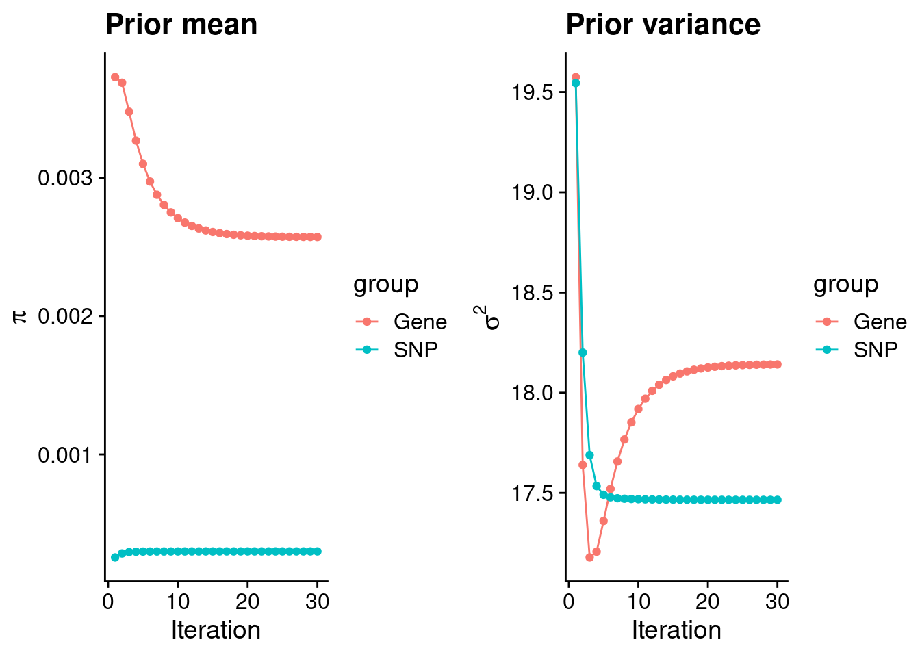
#estimated group prior
estimated_group_prior <- group_prior_rec[,ncol(group_prior_rec)]
names(estimated_group_prior) <- c("gene", "snp")
estimated_group_prior["snp"] <- estimated_group_prior["snp"]*thin #adjust parameter to account for thin argument
print(estimated_group_prior)
gene snp
0.002571585 0.000299628 #estimated group prior variance
estimated_group_prior_var <- group_prior_var_rec[,ncol(group_prior_var_rec)]
names(estimated_group_prior_var) <- c("gene", "snp")
print(estimated_group_prior_var) gene snp
18.14120 17.46535 #report sample size
print(sample_size)[1] 336107#report group size
group_size <- c(nrow(ctwas_gene_res), n_snps)
print(group_size)[1] 11538 7535010#estimated group PVE
estimated_group_pve <- estimated_group_prior_var*estimated_group_prior*group_size/sample_size #check PVE calculation
names(estimated_group_pve) <- c("gene", "snp")
print(estimated_group_pve) gene snp
0.001601474 0.117318375 #compare sum(PIP*mu2/sample_size) with above PVE calculation
c(sum(ctwas_gene_res$PVE),sum(ctwas_snp_res$PVE))[1] 0.2005197 15.2163902Genes with highest PIPs
#distribution of PIPs
hist(ctwas_gene_res$susie_pip, xlim=c(0,1), main="Distribution of Gene PIPs")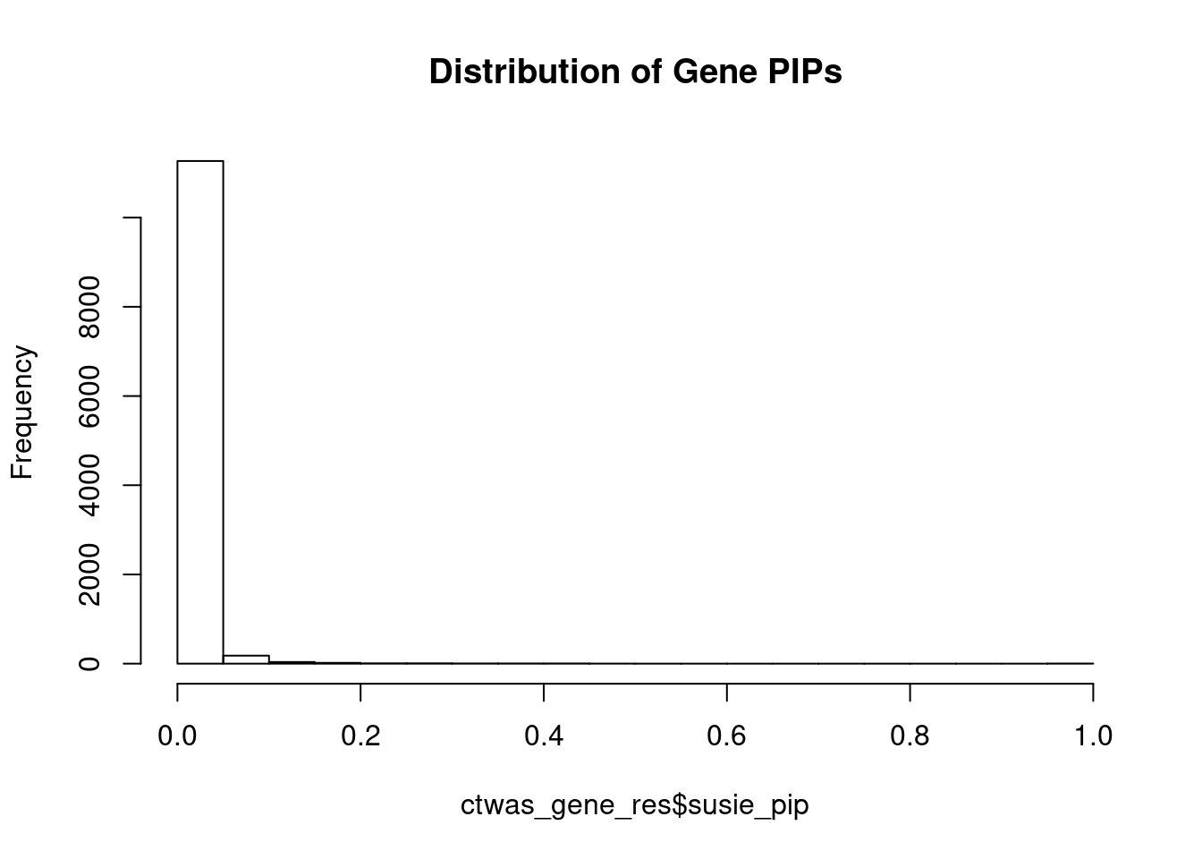
#genes with PIP>0.8 or 20 highest PIPs
head(ctwas_gene_res[order(-ctwas_gene_res$susie_pip),report_cols], max(sum(ctwas_gene_res$susie_pip>0.8), 20))
genename region_tag susie_pip mu2 PVE z
4862 HEY2 6_84 1.0000000 34549.59805 1.027934e-01 5.033965
8605 MRPL1 4_52 0.9999963 16661.35849 4.957141e-02 3.486435
1577 ASCC2 22_10 0.9936907 9364.23192 2.768508e-02 -2.618175
3408 CCND2 12_4 0.8929292 28.66336 7.614942e-05 -5.119990
10379 SP1 12_33 0.7523004 25.56065 5.721181e-05 -4.719016
12572 ETV5 3_114 0.6940969 94.99074 1.961660e-04 9.862284
5598 C18orf8 18_12 0.6056280 55.44443 9.990480e-05 7.499899
13830 HIST1H2BE 6_20 0.4700979 30.74571 4.300267e-05 -6.515410
13559 CTC-498M16.4 5_52 0.4675212 53.74913 7.476446e-05 7.705884
6002 ECE2 3_113 0.4447126 29.33132 3.880910e-05 -5.302197
10039 KCNB2 8_53 0.4401104 64.90303 8.498632e-05 -8.225507
1258 KIF16B 20_12 0.4271436 24.80066 3.151807e-05 -4.619896
12886 AP006621.5 11_1 0.4133098 25.00794 3.075219e-05 -4.506344
7888 YWHAZ 8_69 0.3636711 24.51773 2.652843e-05 4.235328
8734 ELP5 17_6 0.3633053 34.12316 3.688445e-05 4.157351
1722 DNAJC5 20_38 0.3632462 23.94724 2.588088e-05 -4.017824
5697 IGLON5 19_35 0.3603914 31.09134 3.333775e-05 -5.403343
1031 IGSF9B 11_83 0.3492111 29.77714 3.093809e-05 2.128452
5546 CDH13 16_46 0.3484128 24.86130 2.577154e-05 -4.826363
11928 HRAT92 7_1 0.3483643 31.52666 3.267638e-05 -3.948331
num_eqtl
4862 1
8605 1
1577 1
3408 1
10379 1
12572 1
5598 2
13830 1
13559 1
6002 1
10039 1
1258 1
12886 1
7888 1
8734 2
1722 1
5697 1
1031 1
5546 1
11928 3Genes with largest effect sizes
#plot PIP vs effect size
plot(ctwas_gene_res$susie_pip, ctwas_gene_res$mu2, xlab="PIP", ylab="mu^2", main="Gene PIPs vs Effect Size")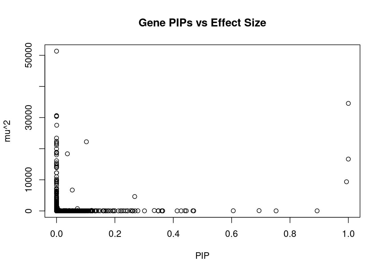
#genes with 20 largest effect sizes
head(ctwas_gene_res[order(-ctwas_gene_res$mu2),report_cols],20)
genename region_tag susie_pip mu2 PVE z
7909 CCDC171 9_13 0.000000000 51332.59 0.000000e+00 7.979137
4862 HEY2 6_84 0.999999990 34549.60 1.027934e-01 5.033965
9691 STX19 3_59 0.000000000 30626.13 0.000000e+00 -5.059656
10446 GSAP 7_49 0.000000000 30470.76 0.000000e+00 5.259703
13068 RP11-490G2.2 1_60 0.000000000 30364.43 0.000000e+00 5.044019
8151 LEO1 15_21 0.000551697 27533.18 4.519385e-05 4.602678
5468 MFAP1 15_16 0.000000000 23395.59 0.000000e+00 4.302998
4567 IGHMBP2 11_38 0.000000000 22373.50 0.000000e+00 -4.327505
13777 LINC02019 3_35 0.102353978 22218.87 6.766267e-03 -4.489974
5290 TMOD3 15_21 0.000000000 21923.04 0.000000e+00 -5.411998
11916 CKMT1A 15_16 0.000000000 21583.23 0.000000e+00 -4.115094
1364 WDR76 15_16 0.000000000 21089.81 0.000000e+00 4.775113
2991 CISH 3_35 0.000000000 19958.31 0.000000e+00 -3.798838
1222 C3orf18 3_35 0.000000000 18831.48 0.000000e+00 4.681781
2990 HEMK1 3_35 0.000000000 18831.48 0.000000e+00 -4.681781
3137 PLCL1 2_117 0.000000000 18556.29 0.000000e+00 5.641781
1064 CCNT2 2_80 0.037246905 18352.47 2.033795e-03 3.685900
2179 PDE4C 19_14 0.000000000 18026.01 0.000000e+00 6.593525
8605 MRPL1 4_52 0.999996266 16661.36 4.957141e-02 3.486435
5185 TUBGCP4 15_16 0.000000000 16113.40 0.000000e+00 3.549755
num_eqtl
7909 1
4862 1
9691 1
10446 1
13068 1
8151 1
5468 1
4567 2
13777 1
5290 1
11916 1
1364 2
2991 1
1222 1
2990 1
3137 1
1064 1
2179 1
8605 1
5185 2Genes with highest PVE
#genes with 20 highest pve
head(ctwas_gene_res[order(-ctwas_gene_res$PVE),report_cols],20)
genename region_tag susie_pip mu2 PVE z
4862 HEY2 6_84 0.999999990 34549.59805 1.027934e-01 5.033965
8605 MRPL1 4_52 0.999996266 16661.35849 4.957141e-02 3.486435
1577 ASCC2 22_10 0.993690700 9364.23192 2.768508e-02 -2.618175
13777 LINC02019 3_35 0.102353978 22218.86934 6.766267e-03 -4.489974
3071 LANCL1 2_124 0.267843315 4621.80894 3.683115e-03 -3.534889
1064 CCNT2 2_80 0.037246905 18352.47006 2.033795e-03 3.685900
7733 MFSD8 4_84 0.053940655 6711.43827 1.077096e-03 2.512064
12572 ETV5 3_114 0.694096889 94.99074 1.961660e-04 9.862284
10923 TTC30B 2_107 0.071465298 738.10105 1.569399e-04 -3.137443
11912 VPS52 6_28 0.334931364 122.68343 1.222543e-04 1.606101
5598 C18orf8 18_12 0.605628049 55.44443 9.990480e-05 7.499899
10039 KCNB2 8_53 0.440110354 64.90303 8.498632e-05 -8.225507
3408 CCND2 12_4 0.892929201 28.66336 7.614942e-05 -5.119990
13559 CTC-498M16.4 5_52 0.467521204 53.74913 7.476446e-05 7.705884
179 NISCH 3_36 0.119991924 169.37244 6.046683e-05 4.468118
6862 GPR61 1_67 0.253910668 78.14077 5.903113e-05 8.755235
10379 SP1 12_33 0.752300392 25.56065 5.721181e-05 -4.719016
8151 LEO1 15_21 0.000551697 27533.17584 4.519385e-05 4.602678
13830 HIST1H2BE 6_20 0.470097948 30.74571 4.300267e-05 -6.515410
6002 ECE2 3_113 0.444712642 29.33132 3.880910e-05 -5.302197
num_eqtl
4862 1
8605 1
1577 1
13777 1
3071 1
1064 1
7733 1
12572 1
10923 1
11912 1
5598 2
10039 1
3408 1
13559 1
179 2
6862 1
10379 1
8151 1
13830 1
6002 1Genes with largest z scores
#genes with 20 largest z scores
head(ctwas_gene_res[order(-abs(ctwas_gene_res$z)),report_cols],20)
genename region_tag susie_pip mu2 PVE z
7736 MST1R 3_35 2.778368e-03 1066.54212 8.816379e-06 -12.646197
38 RBM6 3_35 3.659374e-04 898.09563 9.778040e-07 12.536042
9298 KCTD13 16_24 3.260224e-02 111.56645 1.082190e-05 11.490673
5215 ADCY3 2_16 5.213089e-05 181.05503 2.808201e-08 10.986823
7732 RNF123 3_35 4.331535e-12 814.76736 1.050021e-14 -10.959165
1846 MAPK3 16_24 6.198097e-03 99.06129 1.826774e-06 10.880016
8639 INO80E 16_24 7.196095e-03 95.02103 2.034413e-06 10.733559
12763 RP11-1348G14.4 16_23 7.269926e-02 92.18324 1.993905e-05 10.676318
11175 NPIPB6 16_23 6.407482e-02 94.14672 1.794796e-05 -10.506225
10711 CLN3 16_23 3.078981e-02 89.34064 8.184242e-06 10.452595
9418 NUPR1 16_23 7.177856e-02 98.60480 2.105791e-05 -10.436769
9502 NFATC2IP 16_23 2.728712e-02 87.47261 7.101535e-06 -10.013408
8296 ZNF668 16_24 3.290834e-02 78.12631 7.649372e-06 10.000364
8995 C1QTNF4 11_29 7.823413e-03 95.03242 2.212027e-06 9.961383
12572 ETV5 3_114 6.940969e-01 94.99074 1.961660e-04 9.862284
1938 KAT8 16_24 6.257505e-03 74.20396 1.381499e-06 -9.848191
11718 NDUFS3 11_29 4.101137e-03 85.98951 1.049234e-06 -9.624203
11003 SULT1A2 16_23 8.562947e-03 77.50311 1.974535e-06 -9.620582
11724 LAT 16_23 5.360090e-02 86.33720 1.376869e-05 -9.552834
2577 MTCH2 11_29 3.824449e-03 84.26680 9.588436e-07 -9.551496
num_eqtl
7736 3
38 1
9298 1
5215 2
7732 1
1846 1
8639 1
12763 1
11175 1
10711 1
9418 2
9502 1
8296 1
8995 2
12572 1
1938 1
11718 1
11003 2
11724 1
2577 1Comparing z scores and PIPs
#set nominal signifiance threshold for z scores
alpha <- 0.05

#bonferroni adjusted threshold for z scores
sig_thresh <- qnorm(1-(alpha/nrow(ctwas_gene_res)/2), lower=T)

#Q-Q plot for z scores
obs_z <- ctwas_gene_res$z[order(ctwas_gene_res$z)]
exp_z <- qnorm((1:nrow(ctwas_gene_res))/nrow(ctwas_gene_res))

plot(exp_z, obs_z, xlab="Expected z", ylab="Observed z", main="Gene z score Q-Q plot")
abline(a=0,b=1)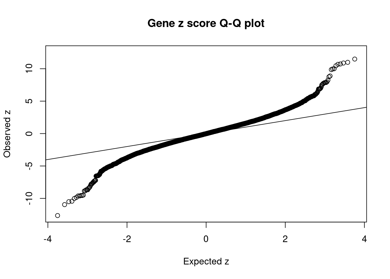
#plot z score vs PIP
plot(abs(ctwas_gene_res$z), ctwas_gene_res$susie_pip, xlab="abs(z)", ylab="PIP")
abline(v=sig_thresh, col="red", lty=2)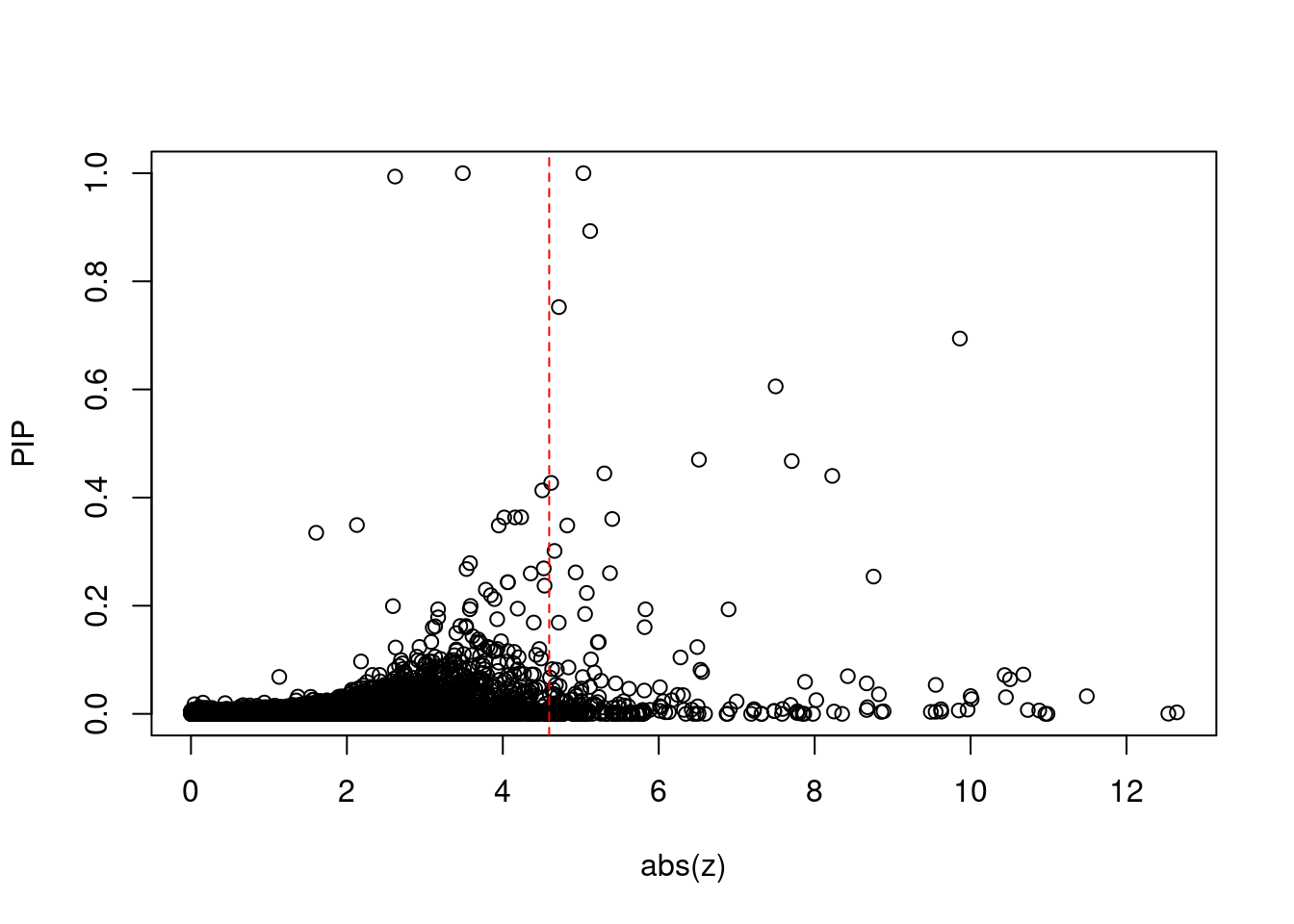
#proportion of significant z scores
mean(abs(ctwas_gene_res$z) > sig_thresh)
[1] 0.0208875#genes with most significant z scores
head(ctwas_gene_res[order(-abs(ctwas_gene_res$z)),report_cols],20) genename region_tag susie_pip mu2 PVE z
7736 MST1R 3_35 2.778368e-03 1066.54212 8.816379e-06 -12.646197
38 RBM6 3_35 3.659374e-04 898.09563 9.778040e-07 12.536042
9298 KCTD13 16_24 3.260224e-02 111.56645 1.082190e-05 11.490673
5215 ADCY3 2_16 5.213089e-05 181.05503 2.808201e-08 10.986823
7732 RNF123 3_35 4.331535e-12 814.76736 1.050021e-14 -10.959165
1846 MAPK3 16_24 6.198097e-03 99.06129 1.826774e-06 10.880016
8639 INO80E 16_24 7.196095e-03 95.02103 2.034413e-06 10.733559
12763 RP11-1348G14.4 16_23 7.269926e-02 92.18324 1.993905e-05 10.676318
11175 NPIPB6 16_23 6.407482e-02 94.14672 1.794796e-05 -10.506225
10711 CLN3 16_23 3.078981e-02 89.34064 8.184242e-06 10.452595
9418 NUPR1 16_23 7.177856e-02 98.60480 2.105791e-05 -10.436769
9502 NFATC2IP 16_23 2.728712e-02 87.47261 7.101535e-06 -10.013408
8296 ZNF668 16_24 3.290834e-02 78.12631 7.649372e-06 10.000364
8995 C1QTNF4 11_29 7.823413e-03 95.03242 2.212027e-06 9.961383
12572 ETV5 3_114 6.940969e-01 94.99074 1.961660e-04 9.862284
1938 KAT8 16_24 6.257505e-03 74.20396 1.381499e-06 -9.848191
11718 NDUFS3 11_29 4.101137e-03 85.98951 1.049234e-06 -9.624203
11003 SULT1A2 16_23 8.562947e-03 77.50311 1.974535e-06 -9.620582
11724 LAT 16_23 5.360090e-02 86.33720 1.376869e-05 -9.552834
2577 MTCH2 11_29 3.824449e-03 84.26680 9.588436e-07 -9.551496
num_eqtl
7736 3
38 1
9298 1
5215 2
7732 1
1846 1
8639 1
12763 1
11175 1
10711 1
9418 2
9502 1
8296 1
8995 2
12572 1
1938 1
11718 1
11003 2
11724 1
2577 1Sensitivity, specificity and precision for silver standard genes
library("readxl")

known_annotations <- read_xlsx("data/summary_known_genes_annotations.xlsx", sheet="BMI")
known_annotations <- unique(known_annotations$`Gene Symbol`)

unrelated_genes <- ctwas_gene_res$genename[!(ctwas_gene_res$genename %in% known_annotations)]

#number of genes in known annotations
print(length(known_annotations))
[1] 41#number of genes in known annotations with imputed expression
print(sum(known_annotations %in% ctwas_gene_res$genename))[1] 24#assign ctwas, TWAS, and bystander genes
ctwas_genes <- ctwas_gene_res$genename[ctwas_gene_res$susie_pip>0.8]
twas_genes <- ctwas_gene_res$genename[abs(ctwas_gene_res$z)>sig_thresh]
novel_genes <- ctwas_genes[!(ctwas_genes %in% twas_genes)]
#significance threshold for TWAS
print(sig_thresh)[1] 4.59471#number of ctwas genes
length(ctwas_genes)[1] 4#number of TWAS genes
length(twas_genes)[1] 241#show novel genes (ctwas genes with not in TWAS genes)
ctwas_gene_res[ctwas_gene_res$genename %in% novel_genes,report_cols] genename region_tag susie_pip mu2 PVE z num_eqtl
8605 MRPL1 4_52 0.9999963 16661.358 0.04957141 3.486435 1
1577 ASCC2 22_10 0.9936907 9364.232 0.02768508 -2.618175 1#sensitivity / recall
sensitivity <- rep(NA,2)
names(sensitivity) <- c("ctwas", "TWAS")
sensitivity["ctwas"] <- sum(ctwas_genes %in% known_annotations)/length(known_annotations)
sensitivity["TWAS"] <- sum(twas_genes %in% known_annotations)/length(known_annotations)
sensitivity ctwas TWAS
0.00000000 0.09756098 #specificity
specificity <- rep(NA,2)
names(specificity) <- c("ctwas", "TWAS")
specificity["ctwas"] <- sum(!(unrelated_genes %in% ctwas_genes))/length(unrelated_genes)
specificity["TWAS"] <- sum(!(unrelated_genes %in% twas_genes))/length(unrelated_genes)
specificity ctwas TWAS
0.9996526 0.9794164 #precision / PPV
precision <- rep(NA,2)
names(precision) <- c("ctwas", "TWAS")
precision["ctwas"] <- sum(ctwas_genes %in% known_annotations)/length(ctwas_genes)
precision["TWAS"] <- sum(twas_genes %in% known_annotations)/length(twas_genes)
precision ctwas TWAS
0.00000000 0.01659751 #ROC curves
pip_range <- (0:1000)/1000
sensitivity <- rep(NA, length(pip_range))
specificity <- rep(NA, length(pip_range))
for (index in 1:length(pip_range)){
pip <- pip_range[index]
ctwas_genes <- ctwas_gene_res$genename[ctwas_gene_res$susie_pip>=pip]
sensitivity[index] <- sum(ctwas_genes %in% known_annotations)/length(known_annotations)
specificity[index] <- sum(!(unrelated_genes %in% ctwas_genes))/length(unrelated_genes)
}
plot(1-specificity, sensitivity, type="l", xlim=c(0,1), ylim=c(0,1))
sig_thresh_range <- seq(from=0, to=max(abs(ctwas_gene_res$z)), length.out=length(pip_range))
for (index in 1:length(sig_thresh_range)){
sig_thresh_plot <- sig_thresh_range[index]
twas_genes <- ctwas_gene_res$genename[abs(ctwas_gene_res$z)>=sig_thresh_plot]
sensitivity[index] <- sum(twas_genes %in% known_annotations)/length(known_annotations)
specificity[index] <- sum(!(unrelated_genes %in% twas_genes))/length(unrelated_genes)
}
lines(1-specificity, sensitivity, xlim=c(0,1), ylim=c(0,1), col="red", lty=2)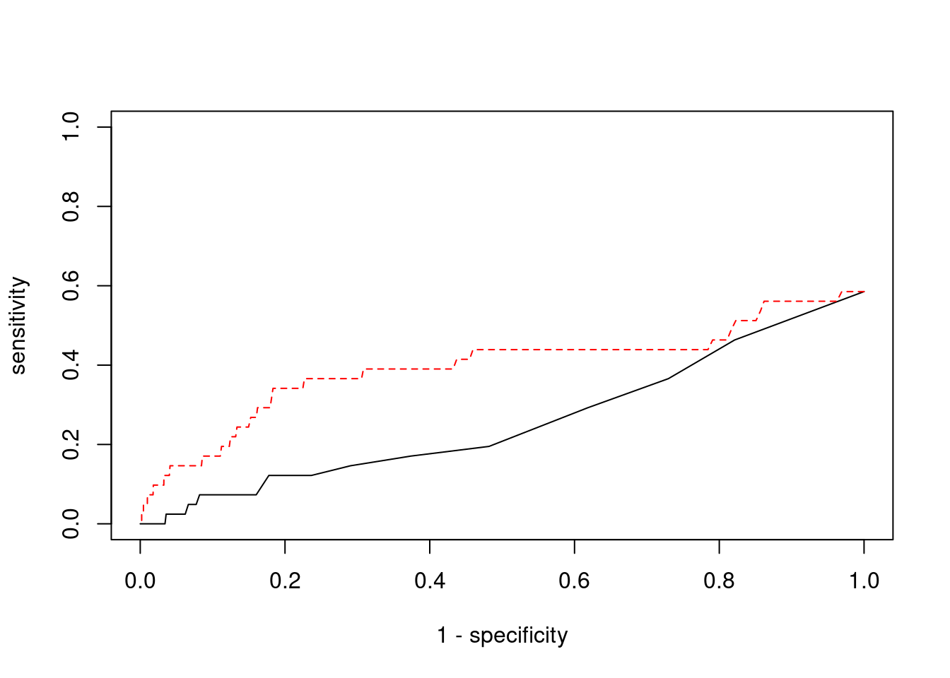
sessionInfo()R version 3.6.1 (2019-07-05)
Platform: x86_64-pc-linux-gnu (64-bit)
Running under: Scientific Linux 7.4 (Nitrogen)
Matrix products: default
BLAS/LAPACK: /software/openblas-0.2.19-el7-x86_64/lib/libopenblas_haswellp-r0.2.19.so
locale:
[1] LC_CTYPE=en_US.UTF-8 LC_NUMERIC=C
[3] LC_TIME=en_US.UTF-8 LC_COLLATE=en_US.UTF-8
[5] LC_MONETARY=en_US.UTF-8 LC_MESSAGES=en_US.UTF-8
[7] LC_PAPER=en_US.UTF-8 LC_NAME=C
[9] LC_ADDRESS=C LC_TELEPHONE=C
[11] LC_MEASUREMENT=en_US.UTF-8 LC_IDENTIFICATION=C
attached base packages:
[1] stats graphics grDevices utils datasets methods base
other attached packages:
[1] readxl_1.3.1 cowplot_1.0.0 ggplot2_3.3.5 workflowr_1.6.2
loaded via a namespace (and not attached):
[1] tidyselect_1.1.1 xfun_0.29 purrr_0.3.4 colorspace_2.0-2
[5] vctrs_0.3.8 generics_0.1.1 htmltools_0.5.2 yaml_2.2.1
[9] utf8_1.2.2 blob_1.2.2 rlang_0.4.12 jquerylib_0.1.4
[13] later_0.8.0 pillar_1.6.4 glue_1.5.1 withr_2.4.3
[17] DBI_1.1.1 bit64_4.0.5 lifecycle_1.0.1 stringr_1.4.0
[21] cellranger_1.1.0 munsell_0.5.0 gtable_0.3.0 evaluate_0.14
[25] memoise_2.0.1 labeling_0.4.2 knitr_1.36 fastmap_1.1.0
[29] httpuv_1.5.1 fansi_0.5.0 highr_0.9 Rcpp_1.0.7
[33] promises_1.0.1 scales_1.1.1 cachem_1.0.6 farver_2.1.0
[37] fs_1.5.2 bit_4.0.4 digest_0.6.29 stringi_1.7.6
[41] dplyr_1.0.7 rprojroot_2.0.2 grid_3.6.1 tools_3.6.1
[45] magrittr_2.0.1 tibble_3.1.6 RSQLite_2.2.8 crayon_1.4.2
[49] whisker_0.3-2 pkgconfig_2.0.3 ellipsis_0.3.2 data.table_1.14.2
[53] assertthat_0.2.1 rmarkdown_2.11 R6_2.5.1 git2r_0.26.1
[57] compiler_3.6.1