BMI - Brain Frontal Cortex BA9
sheng Qian
2021-2-6
Last updated: 2022-02-13
Checks: 6 1
Knit directory: cTWAS_analysis/
This reproducible R Markdown analysis was created with workflowr (version 1.6.2). The Checks tab describes the reproducibility checks that were applied when the results were created. The Past versions tab lists the development history.
Great! Since the R Markdown file has been committed to the Git repository, you know the exact version of the code that produced these results.
Great job! The global environment was empty. Objects defined in the global environment can affect the analysis in your R Markdown file in unknown ways. For reproduciblity it’s best to always run the code in an empty environment.
The command set.seed(20211220) was run prior to running the code in the R Markdown file. Setting a seed ensures that any results that rely on randomness, e.g. subsampling or permutations, are reproducible.
Great job! Recording the operating system, R version, and package versions is critical for reproducibility.
Nice! There were no cached chunks for this analysis, so you can be confident that you successfully produced the results during this run.
Using absolute paths to the files within your workflowr project makes it difficult for you and others to run your code on a different machine. Change the absolute path(s) below to the suggested relative path(s) to make your code more reproducible.
| absolute | relative |
|---|---|
| /project2/xinhe/shengqian/cTWAS/cTWAS_analysis/data/ | data |
| /project2/xinhe/shengqian/cTWAS/cTWAS_analysis/code/ctwas_config.R | code/ctwas_config.R |
Great! You are using Git for version control. Tracking code development and connecting the code version to the results is critical for reproducibility.
The results in this page were generated with repository version 87fee8b. See the Past versions tab to see a history of the changes made to the R Markdown and HTML files.
Note that you need to be careful to ensure that all relevant files for the analysis have been committed to Git prior to generating the results (you can use wflow_publish or wflow_git_commit). workflowr only checks the R Markdown file, but you know if there are other scripts or data files that it depends on. Below is the status of the Git repository when the results were generated:
Ignored files:
    Ignored:    .ipynb_checkpoints/

Untracked files:
    Untracked:  code/.ipynb_checkpoints/
    Untracked:  code/AF_out/
    Untracked:  code/BMI_out/
    Untracked:  code/T2D_out/
    Untracked:  code/ctwas_config.R
    Untracked:  code/mapping.R
    Untracked:  code/out/
    Untracked:  code/run_AF_analysis.sbatch
    Untracked:  code/run_AF_analysis.sh
    Untracked:  code/run_AF_ctwas_rss_LDR.R
    Untracked:  code/run_BMI_analysis.sbatch
    Untracked:  code/run_BMI_analysis.sh
    Untracked:  code/run_BMI_ctwas_rss_LDR.R
    Untracked:  code/run_T2D_analysis.sbatch
    Untracked:  code/run_T2D_analysis.sh
    Untracked:  code/run_T2D_ctwas_rss_LDR.R
    Untracked:  data/.ipynb_checkpoints/
    Untracked:  data/AF/
    Untracked:  data/BMI/
    Untracked:  data/T2D/
    Untracked:  data/UKBB/
    Untracked:  data/UKBB_SNPs_Info.text
    Untracked:  data/gene_OMIM.txt
    Untracked:  data/gene_pip_0.8.txt
    Untracked:  data/mashr_Heart_Atrial_Appendage.db
    Untracked:  data/summary_known_genes_annotations.xlsx
    Untracked:  data/untitled.txt
Note that any generated files, e.g. HTML, png, CSS, etc., are not included in this status report because it is ok for generated content to have uncommitted changes.
These are the previous versions of the repository in which changes were made to the R Markdown (analysis/BMI_Brain_Frontal_Cortex_BA9.Rmd) and HTML (docs/BMI_Brain_Frontal_Cortex_BA9.html) files. If you’ve configured a remote Git repository (see ?wflow_git_remote), click on the hyperlinks in the table below to view the files as they were in that past version.
| File | Version | Author | Date | Message |
|---|---|---|---|---|
| Rmd | 87fee8b | sq-96 | 2022-02-13 | update |
Introduction
Weight QC
qclist_all <- list()

qc_files <- paste0(results_dir, "/", list.files(results_dir, pattern="exprqc.Rd"))

for (i in 1:length(qc_files)){
  load(qc_files[i])
  chr <- unlist(strsplit(rev(unlist(strsplit(qc_files[i], "_")))[1], "[.]"))[1]
  qclist_all[[chr]] <- cbind(do.call(rbind, lapply(qclist,unlist)), as.numeric(substring(chr,4)))
}

qclist_all <- data.frame(do.call(rbind, qclist_all))
colnames(qclist_all)[ncol(qclist_all)] <- "chr"

rm(qclist, wgtlist, z_gene_chr)

#number of imputed weights
nrow(qclist_all)
[1] 11472#number of imputed weights by chromosome
table(qclist_all$chr)
   1    2    3    4    5    6    7    8    9   10   11   12   13   14   15   16
1144  832  640  455  556  662  528  439  419  459  689  634  234  371  365  512
  17   18   19   20   21   22
 717  176  886  353  119  282
#number of imputed weights without missing variants
sum(qclist_all$nmiss==0)[1] 8962#proportion of imputed weights without missing variants
mean(qclist_all$nmiss==0)[1] 0.7812064Load ctwas results
Check convergence of parameters
library(ggplot2)
library(cowplot)
********************************************************Note: As of version 1.0.0, cowplot does not change the default ggplot2 theme anymore. To recover the previous behavior, execute:
theme_set(theme_cowplot())********************************************************load(paste0(results_dir, "/", analysis_id, "_ctwas.s2.susieIrssres.Rd"))
df <- data.frame(niter = rep(1:ncol(group_prior_rec), 2),
value = c(group_prior_rec[1,], group_prior_rec[2,]),
group = rep(c("Gene", "SNP"), each = ncol(group_prior_rec)))
df$group <- as.factor(df$group)
df$value[df$group=="SNP"] <- df$value[df$group=="SNP"]*thin #adjust parameter to account for thin argument
p_pi <- ggplot(df, aes(x=niter, y=value, group=group)) +
geom_line(aes(color=group)) +
geom_point(aes(color=group)) +
xlab("Iteration") + ylab(bquote(pi)) +
ggtitle("Prior mean") +
theme_cowplot()
df <- data.frame(niter = rep(1:ncol(group_prior_var_rec), 2),
value = c(group_prior_var_rec[1,], group_prior_var_rec[2,]),
group = rep(c("Gene", "SNP"), each = ncol(group_prior_var_rec)))
df$group <- as.factor(df$group)
p_sigma2 <- ggplot(df, aes(x=niter, y=value, group=group)) +
geom_line(aes(color=group)) +
geom_point(aes(color=group)) +
xlab("Iteration") + ylab(bquote(sigma^2)) +
ggtitle("Prior variance") +
theme_cowplot()
plot_grid(p_pi, p_sigma2)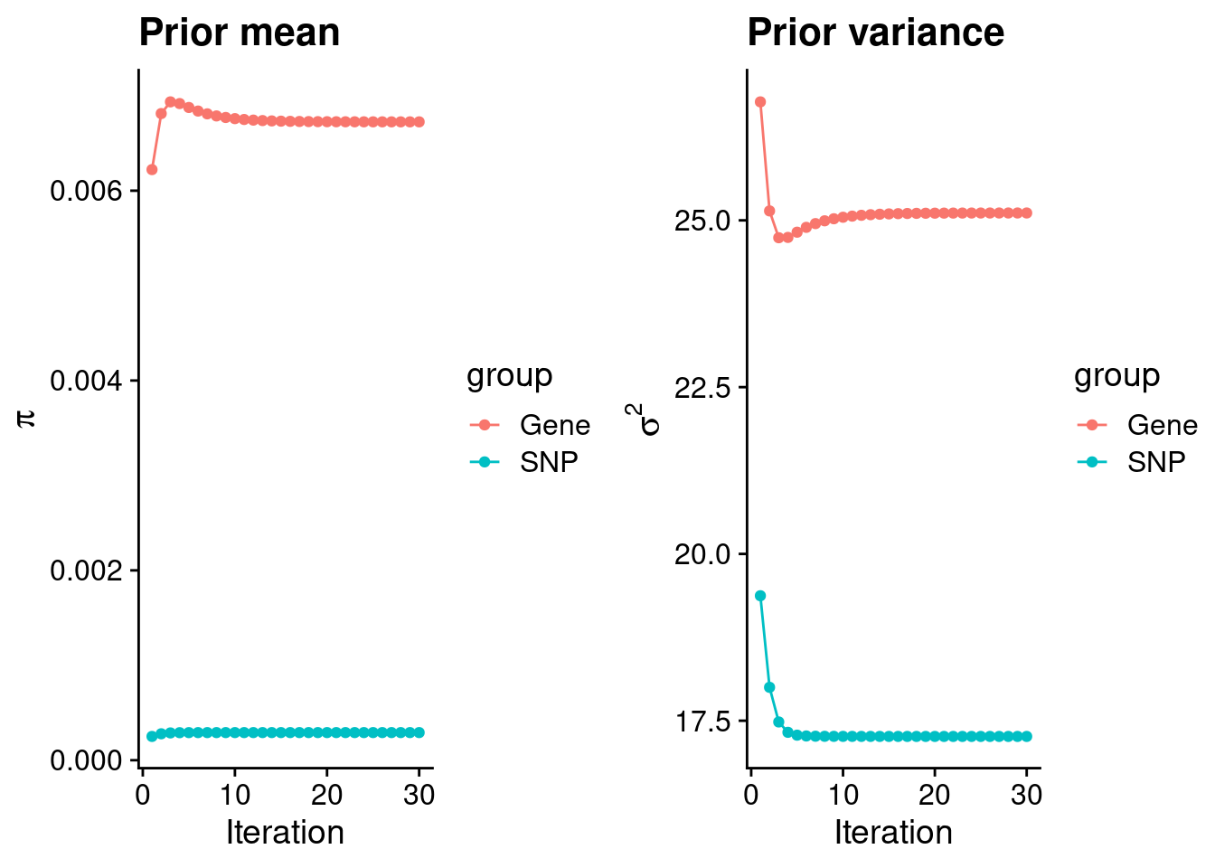
#estimated group prior
estimated_group_prior <- group_prior_rec[,ncol(group_prior_rec)]
names(estimated_group_prior) <- c("gene", "snp")
estimated_group_prior["snp"] <- estimated_group_prior["snp"]*thin #adjust parameter to account for thin argument
print(estimated_group_prior)
gene snp
0.0067252380 0.0002911334 #estimated group prior variance
estimated_group_prior_var <- group_prior_var_rec[,ncol(group_prior_var_rec)]
names(estimated_group_prior_var) <- c("gene", "snp")
print(estimated_group_prior_var) gene snp
25.11067 17.26460 #report sample size
print(sample_size)[1] 336107#report group size
group_size <- c(nrow(ctwas_gene_res), n_snps)
print(group_size)[1] 11472 7535010#estimated group PVE
estimated_group_pve <- estimated_group_prior_var*estimated_group_prior*group_size/sample_size #check PVE calculation
names(estimated_group_pve) <- c("gene", "snp")
print(estimated_group_pve) gene snp
0.005764048 0.112682042 #compare sum(PIP*mu2/sample_size) with above PVE calculation
c(sum(ctwas_gene_res$PVE),sum(ctwas_snp_res$PVE))[1] 0.3711252 15.5332734Genes with highest PIPs
#distribution of PIPs
hist(ctwas_gene_res$susie_pip, xlim=c(0,1), main="Distribution of Gene PIPs")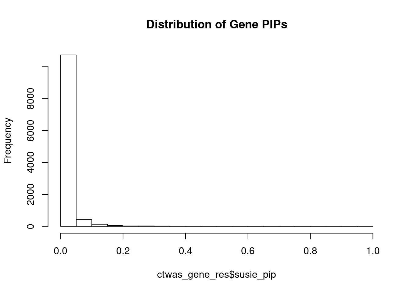
#genes with PIP>0.8 or 20 highest PIPs
head(ctwas_gene_res[order(-ctwas_gene_res$susie_pip),report_cols], max(sum(ctwas_gene_res$susie_pip>0.8), 20))
genename region_tag susie_pip mu2 PVE z
8994 NEGR1 1_46 1.0000000 17779.39337 5.289802e-02 -10.657317
13051 RP11-490G2.2 1_60 1.0000000 33092.91269 9.845946e-02 5.044019
10446 GSAP 7_49 1.0000000 32937.38554 9.799673e-02 5.259703
751 MAPK6 15_21 1.0000000 35089.11318 1.043986e-01 -4.600218
7741 PPM1M 3_36 0.9999999 247.29833 7.357726e-04 4.675362
3673 FLT3 13_7 0.9522768 33.57224 9.511870e-05 -5.359706
979 PIK3C3 18_23 0.9326376 52.81973 1.465654e-04 6.864417
8027 CASP7 10_71 0.8054467 25.18208 6.034633e-05 4.610051
9305 ASPHD1 16_24 0.7995340 119.95832 2.853578e-04 -11.937656
3823 PREX1 20_30 0.7871489 34.78058 8.145469e-05 5.633918
1486 RASSF7 11_1 0.7686828 22.53360 5.153474e-05 3.476827
5622 C18orf8 18_12 0.7674687 60.95167 1.391774e-04 7.723439
5021 DCAF7 17_37 0.7484079 28.87254 6.429036e-05 5.436897
10039 KCNB2 8_53 0.7451725 66.52058 1.474807e-04 -8.225507
12703 CTC-467M3.3 5_52 0.7200174 90.77823 1.944676e-04 9.482167
2989 IFT57 3_67 0.7135486 44.78834 9.508478e-05 -5.822399
13296 AARSD1 17_25 0.7088165 33.53734 7.072694e-05 5.541598
4728 YWHAQ 2_6 0.6955237 26.36178 5.455179e-05 4.910669
6022 ECE2 3_113 0.6950195 29.98887 6.201255e-05 -5.304782
10781 SF3B3 16_37 0.6810625 35.85913 7.266231e-05 -6.852259
num_eqtl
8994 2
13051 1
10446 1
751 1
7741 3
3673 1
979 2
8027 2
9305 1
3823 1
1486 1
5622 3
5021 1
10039 1
12703 1
2989 2
13296 1
4728 1
6022 1
10781 1Genes with largest effect sizes
#plot PIP vs effect size
plot(ctwas_gene_res$susie_pip, ctwas_gene_res$mu2, xlab="PIP", ylab="mu^2", main="Gene PIPs vs Effect Size")
#genes with 20 largest effect sizes
head(ctwas_gene_res[order(-ctwas_gene_res$mu2),report_cols],20)
genename region_tag susie_pip mu2 PVE z
9 SEMA3F 3_35 0.000000e+00 72069.90 0.000000e+00 7.681163
10678 SLC38A3 3_35 0.000000e+00 67358.48 0.000000e+00 6.725828
7734 CAMKV 3_35 0.000000e+00 52493.18 0.000000e+00 -10.226037
7917 CCDC171 9_13 0.000000e+00 50279.36 0.000000e+00 8.023170
1462 MAST3 19_14 0.000000e+00 42245.44 0.000000e+00 6.952564
31 RBM5 3_35 0.000000e+00 42132.93 0.000000e+00 12.473227
41 RBM6 3_35 0.000000e+00 40748.94 0.000000e+00 12.536042
751 MAPK6 15_21 1.000000e+00 35089.11 1.043986e-01 -4.600218
8150 LEO1 15_21 2.603458e-03 34887.56 2.702362e-04 4.602678
13051 RP11-490G2.2 1_60 1.000000e+00 33092.91 9.845946e-02 5.044019
10446 GSAP 7_49 1.000000e+00 32937.39 9.799673e-02 5.259703
6317 CNNM2 10_66 0.000000e+00 31589.44 0.000000e+00 -5.980953
5488 MFAP1 15_16 7.668311e-04 23546.53 5.372161e-05 4.302998
12490 HYPK 15_16 6.638464e-06 23445.18 4.630668e-07 4.322039
7732 RNF123 3_35 0.000000e+00 23052.76 0.000000e+00 -10.957103
11029 MRPL21 11_38 0.000000e+00 22517.24 0.000000e+00 4.215024
1379 WDR76 15_16 0.000000e+00 21366.60 0.000000e+00 4.686940
11910 CKMT1A 15_16 0.000000e+00 21087.36 0.000000e+00 4.129652
9680 DHFR2 3_59 0.000000e+00 17795.96 0.000000e+00 3.265951
8994 NEGR1 1_46 1.000000e+00 17779.39 5.289802e-02 -10.657317
num_eqtl
9 1
10678 1
7734 2
7917 2
1462 2
31 1
41 1
751 1
8150 1
13051 1
10446 1
6317 2
5488 1
12490 1
7732 1
11029 2
1379 2
11910 1
9680 3
8994 2Genes with highest PVE
#genes with 20 highest pve
head(ctwas_gene_res[order(-ctwas_gene_res$PVE),report_cols],20)
genename region_tag susie_pip mu2 PVE z
751 MAPK6 15_21 1.000000000 35089.11318 1.043986e-01 -4.600218
13051 RP11-490G2.2 1_60 1.000000000 33092.91269 9.845946e-02 5.044019
10446 GSAP 7_49 1.000000000 32937.38554 9.799673e-02 5.259703
8994 NEGR1 1_46 1.000000000 17779.39337 5.289802e-02 -10.657317
10925 TTC30B 2_107 0.349013321 762.39335 7.916688e-04 -3.137443
7741 PPM1M 3_36 0.999999902 247.29833 7.357726e-04 4.675362
3029 SPCS1 3_36 0.516680612 361.49123 5.557025e-04 -5.066891
9305 ASPHD1 16_24 0.799534046 119.95832 2.853578e-04 -11.937656
8150 LEO1 15_21 0.002603458 34887.55835 2.702362e-04 4.602678
12703 CTC-467M3.3 5_52 0.720017429 90.77823 1.944676e-04 9.482167
10039 KCNB2 8_53 0.745172489 66.52058 1.474807e-04 -8.225507
979 PIK3C3 18_23 0.932637599 52.81973 1.465654e-04 6.864417
5622 C18orf8 18_12 0.767468679 60.95167 1.391774e-04 7.723439
6868 GPR61 1_67 0.582831591 80.07469 1.388548e-04 8.755235
8172 MC4R 18_34 0.344096083 130.49766 1.335995e-04 13.311794
5343 G3BP2 4_51 0.360464481 121.37899 1.301753e-04 -2.133639
7387 TAL1 1_29 0.666871581 48.91502 9.705253e-05 -6.744974
3673 FLT3 13_7 0.952276779 33.57224 9.511870e-05 -5.359706
2989 IFT57 3_67 0.713548587 44.78834 9.508478e-05 -5.822399
5424 SUOX 12_35 0.519005045 58.30476 9.003224e-05 -5.806919
num_eqtl
751 1
13051 1
10446 1
8994 2
10925 1
7741 3
3029 1
9305 1
8150 1
12703 1
10039 1
979 2
5622 3
6868 1
8172 1
5343 1
7387 2
3673 1
2989 2
5424 1Genes with largest z scores
#genes with 20 largest z scores
head(ctwas_gene_res[order(-abs(ctwas_gene_res$z)),report_cols],20)
genename region_tag susie_pip mu2 PVE z
8172 MC4R 18_34 0.344096083 130.49766 1.335995e-04 13.311794
41 RBM6 3_35 0.000000000 40748.93779 0.000000e+00 12.536042
31 RBM5 3_35 0.000000000 42132.93474 0.000000e+00 12.473227
9305 ASPHD1 16_24 0.799534046 119.95832 2.853578e-04 -11.937656
6407 TAOK2 16_24 0.051557591 125.43653 1.924151e-05 11.848686
7736 MST1R 3_35 0.000000000 6793.57015 0.000000e+00 -11.803377
9306 KCTD13 16_24 0.033410814 112.45110 1.117823e-05 11.490673
9304 SEZ6L2 16_24 0.020286967 110.70293 6.681880e-06 -11.407378
7732 RNF123 3_35 0.000000000 23052.75535 0.000000e+00 -10.957103
8634 INO80E 16_24 0.023303794 98.35711 6.819536e-06 10.794453
8994 NEGR1 1_46 1.000000000 17779.39337 5.289802e-02 -10.657317
10707 CLN3 16_23 0.089642016 68.18511 1.818543e-05 10.452595
7734 CAMKV 3_35 0.000000000 52493.17731 0.000000e+00 -10.226037
12221 RP11-196G11.6 16_24 0.336709511 81.08744 8.123280e-05 10.127704
11002 SULT1A2 16_23 0.040749579 64.25940 7.790803e-06 -10.075303
12241 NPIPB7 16_23 0.029321556 65.40877 5.706179e-06 10.037986
8290 ZNF646 16_24 0.081104970 77.81042 1.877620e-05 -10.000364
2891 COL4A3BP 5_44 0.022153965 72.01389 4.746682e-06 -9.828145
10737 SKOR1 15_31 0.542610035 52.50453 8.476314e-05 -9.635319
8993 C1QTNF4 11_29 0.008762151 87.67096 2.285541e-06 9.563515
num_eqtl
8172 1
41 1
31 1
9305 1
6407 1
7736 2
9306 1
9304 1
7732 1
8634 2
8994 2
10707 1
7734 2
12221 1
11002 2
12241 1
8290 1
2891 1
10737 1
8993 1Comparing z scores and PIPs
#set nominal signifiance threshold for z scores
alpha <- 0.05

#bonferroni adjusted threshold for z scores
sig_thresh <- qnorm(1-(alpha/nrow(ctwas_gene_res)/2), lower=T)

#Q-Q plot for z scores
obs_z <- ctwas_gene_res$z[order(ctwas_gene_res$z)]
exp_z <- qnorm((1:nrow(ctwas_gene_res))/nrow(ctwas_gene_res))

plot(exp_z, obs_z, xlab="Expected z", ylab="Observed z", main="Gene z score Q-Q plot")
abline(a=0,b=1)
#plot z score vs PIP
plot(abs(ctwas_gene_res$z), ctwas_gene_res$susie_pip, xlab="abs(z)", ylab="PIP")
abline(v=sig_thresh, col="red", lty=2)
#proportion of significant z scores
mean(abs(ctwas_gene_res$z) > sig_thresh)
[1] 0.02222803#genes with most significant z scores
head(ctwas_gene_res[order(-abs(ctwas_gene_res$z)),report_cols],20) genename region_tag susie_pip mu2 PVE z
8172 MC4R 18_34 0.344096083 130.49766 1.335995e-04 13.311794
41 RBM6 3_35 0.000000000 40748.93779 0.000000e+00 12.536042
31 RBM5 3_35 0.000000000 42132.93474 0.000000e+00 12.473227
9305 ASPHD1 16_24 0.799534046 119.95832 2.853578e-04 -11.937656
6407 TAOK2 16_24 0.051557591 125.43653 1.924151e-05 11.848686
7736 MST1R 3_35 0.000000000 6793.57015 0.000000e+00 -11.803377
9306 KCTD13 16_24 0.033410814 112.45110 1.117823e-05 11.490673
9304 SEZ6L2 16_24 0.020286967 110.70293 6.681880e-06 -11.407378
7732 RNF123 3_35 0.000000000 23052.75535 0.000000e+00 -10.957103
8634 INO80E 16_24 0.023303794 98.35711 6.819536e-06 10.794453
8994 NEGR1 1_46 1.000000000 17779.39337 5.289802e-02 -10.657317
10707 CLN3 16_23 0.089642016 68.18511 1.818543e-05 10.452595
7734 CAMKV 3_35 0.000000000 52493.17731 0.000000e+00 -10.226037
12221 RP11-196G11.6 16_24 0.336709511 81.08744 8.123280e-05 10.127704
11002 SULT1A2 16_23 0.040749579 64.25940 7.790803e-06 -10.075303
12241 NPIPB7 16_23 0.029321556 65.40877 5.706179e-06 10.037986
8290 ZNF646 16_24 0.081104970 77.81042 1.877620e-05 -10.000364
2891 COL4A3BP 5_44 0.022153965 72.01389 4.746682e-06 -9.828145
10737 SKOR1 15_31 0.542610035 52.50453 8.476314e-05 -9.635319
8993 C1QTNF4 11_29 0.008762151 87.67096 2.285541e-06 9.563515
num_eqtl
8172 1
41 1
31 1
9305 1
6407 1
7736 2
9306 1
9304 1
7732 1
8634 2
8994 2
10707 1
7734 2
12221 1
11002 2
12241 1
8290 1
2891 1
10737 1
8993 1Sensitivity, specificity and precision for silver standard genes
library("readxl")

known_annotations <- read_xlsx("data/summary_known_genes_annotations.xlsx", sheet="BMI")
known_annotations <- unique(known_annotations$`Gene Symbol`)

unrelated_genes <- ctwas_gene_res$genename[!(ctwas_gene_res$genename %in% known_annotations)]

#number of genes in known annotations
print(length(known_annotations))
[1] 41#number of genes in known annotations with imputed expression
print(sum(known_annotations %in% ctwas_gene_res$genename))[1] 26#assign ctwas, TWAS, and bystander genes
ctwas_genes <- ctwas_gene_res$genename[ctwas_gene_res$susie_pip>0.8]
twas_genes <- ctwas_gene_res$genename[abs(ctwas_gene_res$z)>sig_thresh]
novel_genes <- ctwas_genes[!(ctwas_genes %in% twas_genes)]
#significance threshold for TWAS
print(sig_thresh)[1] 4.593514#number of ctwas genes
length(ctwas_genes)[1] 8#number of TWAS genes
length(twas_genes)[1] 255#show novel genes (ctwas genes with not in TWAS genes)
ctwas_gene_res[ctwas_gene_res$genename %in% novel_genes,report_cols][1] genename region_tag susie_pip mu2 PVE z num_eqtl
<0 rows> (or 0-length row.names)#sensitivity / recall
sensitivity <- rep(NA,2)
names(sensitivity) <- c("ctwas", "TWAS")
sensitivity["ctwas"] <- sum(ctwas_genes %in% known_annotations)/length(known_annotations)
sensitivity["TWAS"] <- sum(twas_genes %in% known_annotations)/length(known_annotations)
sensitivity ctwas TWAS
0.02439024 0.12195122 #specificity
specificity <- rep(NA,2)
names(specificity) <- c("ctwas", "TWAS")
specificity["ctwas"] <- sum(!(unrelated_genes %in% ctwas_genes))/length(unrelated_genes)
specificity["TWAS"] <- sum(!(unrelated_genes %in% twas_genes))/length(unrelated_genes)
specificity ctwas TWAS
0.9993884 0.9781583 #precision / PPV
precision <- rep(NA,2)
names(precision) <- c("ctwas", "TWAS")
precision["ctwas"] <- sum(ctwas_genes %in% known_annotations)/length(ctwas_genes)
precision["TWAS"] <- sum(twas_genes %in% known_annotations)/length(twas_genes)
precision ctwas TWAS
0.12500000 0.01960784 #ROC curves
pip_range <- (0:1000)/1000
sensitivity <- rep(NA, length(pip_range))
specificity <- rep(NA, length(pip_range))
for (index in 1:length(pip_range)){
pip <- pip_range[index]
ctwas_genes <- ctwas_gene_res$genename[ctwas_gene_res$susie_pip>=pip]
sensitivity[index] <- sum(ctwas_genes %in% known_annotations)/length(known_annotations)
specificity[index] <- sum(!(unrelated_genes %in% ctwas_genes))/length(unrelated_genes)
}
plot(1-specificity, sensitivity, type="l", xlim=c(0,1), ylim=c(0,1))
sig_thresh_range <- seq(from=0, to=max(abs(ctwas_gene_res$z)), length.out=length(pip_range))
for (index in 1:length(sig_thresh_range)){
sig_thresh_plot <- sig_thresh_range[index]
twas_genes <- ctwas_gene_res$genename[abs(ctwas_gene_res$z)>=sig_thresh_plot]
sensitivity[index] <- sum(twas_genes %in% known_annotations)/length(known_annotations)
specificity[index] <- sum(!(unrelated_genes %in% twas_genes))/length(unrelated_genes)
}
lines(1-specificity, sensitivity, xlim=c(0,1), ylim=c(0,1), col="red", lty=2)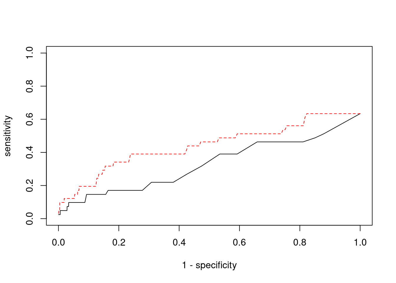
sessionInfo()R version 3.6.1 (2019-07-05)
Platform: x86_64-pc-linux-gnu (64-bit)
Running under: Scientific Linux 7.4 (Nitrogen)
Matrix products: default
BLAS/LAPACK: /software/openblas-0.2.19-el7-x86_64/lib/libopenblas_haswellp-r0.2.19.so
locale:
[1] LC_CTYPE=en_US.UTF-8 LC_NUMERIC=C
[3] LC_TIME=en_US.UTF-8 LC_COLLATE=en_US.UTF-8
[5] LC_MONETARY=en_US.UTF-8 LC_MESSAGES=en_US.UTF-8
[7] LC_PAPER=en_US.UTF-8 LC_NAME=C
[9] LC_ADDRESS=C LC_TELEPHONE=C
[11] LC_MEASUREMENT=en_US.UTF-8 LC_IDENTIFICATION=C
attached base packages:
[1] stats graphics grDevices utils datasets methods base
other attached packages:
[1] readxl_1.3.1 cowplot_1.0.0 ggplot2_3.3.5 workflowr_1.6.2
loaded via a namespace (and not attached):
[1] tidyselect_1.1.1 xfun_0.29 purrr_0.3.4 colorspace_2.0-2
[5] vctrs_0.3.8 generics_0.1.1 htmltools_0.5.2 yaml_2.2.1
[9] utf8_1.2.2 blob_1.2.2 rlang_0.4.12 jquerylib_0.1.4
[13] later_0.8.0 pillar_1.6.4 glue_1.5.1 withr_2.4.3
[17] DBI_1.1.1 bit64_4.0.5 lifecycle_1.0.1 stringr_1.4.0
[21] cellranger_1.1.0 munsell_0.5.0 gtable_0.3.0 evaluate_0.14
[25] memoise_2.0.1 labeling_0.4.2 knitr_1.36 fastmap_1.1.0
[29] httpuv_1.5.1 fansi_0.5.0 highr_0.9 Rcpp_1.0.7
[33] promises_1.0.1 scales_1.1.1 cachem_1.0.6 farver_2.1.0
[37] fs_1.5.2 bit_4.0.4 digest_0.6.29 stringi_1.7.6
[41] dplyr_1.0.7 rprojroot_2.0.2 grid_3.6.1 tools_3.6.1
[45] magrittr_2.0.1 tibble_3.1.6 RSQLite_2.2.8 crayon_1.4.2
[49] whisker_0.3-2 pkgconfig_2.0.3 ellipsis_0.3.2 data.table_1.14.2
[53] assertthat_0.2.1 rmarkdown_2.11 R6_2.5.1 git2r_0.26.1
[57] compiler_3.6.1