BMI - Brain Hippocampus
sheng Qian
2021-2-6
Last updated: 2022-02-13
Checks: 6 1
Knit directory: cTWAS_analysis/
This reproducible R Markdown analysis was created with workflowr (version 1.6.2). The Checks tab describes the reproducibility checks that were applied when the results were created. The Past versions tab lists the development history.
Great! Since the R Markdown file has been committed to the Git repository, you know the exact version of the code that produced these results.
Great job! The global environment was empty. Objects defined in the global environment can affect the analysis in your R Markdown file in unknown ways. For reproduciblity it’s best to always run the code in an empty environment.
The command set.seed(20211220) was run prior to running the code in the R Markdown file. Setting a seed ensures that any results that rely on randomness, e.g. subsampling or permutations, are reproducible.
Great job! Recording the operating system, R version, and package versions is critical for reproducibility.
Nice! There were no cached chunks for this analysis, so you can be confident that you successfully produced the results during this run.
Using absolute paths to the files within your workflowr project makes it difficult for you and others to run your code on a different machine. Change the absolute path(s) below to the suggested relative path(s) to make your code more reproducible.
| absolute | relative |
|---|---|
| /project2/xinhe/shengqian/cTWAS/cTWAS_analysis/data/ | data |
| /project2/xinhe/shengqian/cTWAS/cTWAS_analysis/code/ctwas_config.R | code/ctwas_config.R |
Great! You are using Git for version control. Tracking code development and connecting the code version to the results is critical for reproducibility.
The results in this page were generated with repository version 87fee8b. See the Past versions tab to see a history of the changes made to the R Markdown and HTML files.
Note that you need to be careful to ensure that all relevant files for the analysis have been committed to Git prior to generating the results (you can use wflow_publish or wflow_git_commit). workflowr only checks the R Markdown file, but you know if there are other scripts or data files that it depends on. Below is the status of the Git repository when the results were generated:
Ignored files:
    Ignored:    .ipynb_checkpoints/

Untracked files:
    Untracked:  code/.ipynb_checkpoints/
    Untracked:  code/AF_out/
    Untracked:  code/BMI_out/
    Untracked:  code/T2D_out/
    Untracked:  code/ctwas_config.R
    Untracked:  code/mapping.R
    Untracked:  code/out/
    Untracked:  code/run_AF_analysis.sbatch
    Untracked:  code/run_AF_analysis.sh
    Untracked:  code/run_AF_ctwas_rss_LDR.R
    Untracked:  code/run_BMI_analysis.sbatch
    Untracked:  code/run_BMI_analysis.sh
    Untracked:  code/run_BMI_ctwas_rss_LDR.R
    Untracked:  code/run_T2D_analysis.sbatch
    Untracked:  code/run_T2D_analysis.sh
    Untracked:  code/run_T2D_ctwas_rss_LDR.R
    Untracked:  data/.ipynb_checkpoints/
    Untracked:  data/AF/
    Untracked:  data/BMI/
    Untracked:  data/T2D/
    Untracked:  data/UKBB/
    Untracked:  data/UKBB_SNPs_Info.text
    Untracked:  data/gene_OMIM.txt
    Untracked:  data/gene_pip_0.8.txt
    Untracked:  data/mashr_Heart_Atrial_Appendage.db
    Untracked:  data/summary_known_genes_annotations.xlsx
    Untracked:  data/untitled.txt
Note that any generated files, e.g. HTML, png, CSS, etc., are not included in this status report because it is ok for generated content to have uncommitted changes.
These are the previous versions of the repository in which changes were made to the R Markdown (analysis/BMI_Brain_Hippocampus.Rmd) and HTML (docs/BMI_Brain_Hippocampus.html) files. If you’ve configured a remote Git repository (see ?wflow_git_remote), click on the hyperlinks in the table below to view the files as they were in that past version.
| File | Version | Author | Date | Message |
|---|---|---|---|---|
| Rmd | 87fee8b | sq-96 | 2022-02-13 | update |
Introduction
Weight QC
qclist_all <- list()

qc_files <- paste0(results_dir, "/", list.files(results_dir, pattern="exprqc.Rd"))

for (i in 1:length(qc_files)){
  load(qc_files[i])
  chr <- unlist(strsplit(rev(unlist(strsplit(qc_files[i], "_")))[1], "[.]"))[1]
  qclist_all[[chr]] <- cbind(do.call(rbind, lapply(qclist,unlist)), as.numeric(substring(chr,4)))
}

qclist_all <- data.frame(do.call(rbind, qclist_all))
colnames(qclist_all)[ncol(qclist_all)] <- "chr"

rm(qclist, wgtlist, z_gene_chr)

#number of imputed weights
nrow(qclist_all)
[1] 10973#number of imputed weights by chromosome
table(qclist_all$chr)
   1    2    3    4    5    6    7    8    9   10   11   12   13   14   15   16
1076  769  643  427  529  614  510  402  415  437  663  585  220  377  370  516
  17   18   19   20   21   22
 664  166  865  330  117  278
#number of imputed weights without missing variants
sum(qclist_all$nmiss==0)[1] 8798#proportion of imputed weights without missing variants
mean(qclist_all$nmiss==0)[1] 0.8017862Load ctwas results
Check convergence of parameters
library(ggplot2)
library(cowplot)
********************************************************Note: As of version 1.0.0, cowplot does not change the default ggplot2 theme anymore. To recover the previous behavior, execute:
theme_set(theme_cowplot())********************************************************load(paste0(results_dir, "/", analysis_id, "_ctwas.s2.susieIrssres.Rd"))
df <- data.frame(niter = rep(1:ncol(group_prior_rec), 2),
value = c(group_prior_rec[1,], group_prior_rec[2,]),
group = rep(c("Gene", "SNP"), each = ncol(group_prior_rec)))
df$group <- as.factor(df$group)
df$value[df$group=="SNP"] <- df$value[df$group=="SNP"]*thin #adjust parameter to account for thin argument
p_pi <- ggplot(df, aes(x=niter, y=value, group=group)) +
geom_line(aes(color=group)) +
geom_point(aes(color=group)) +
xlab("Iteration") + ylab(bquote(pi)) +
ggtitle("Prior mean") +
theme_cowplot()
df <- data.frame(niter = rep(1:ncol(group_prior_var_rec), 2),
value = c(group_prior_var_rec[1,], group_prior_var_rec[2,]),
group = rep(c("Gene", "SNP"), each = ncol(group_prior_var_rec)))
df$group <- as.factor(df$group)
p_sigma2 <- ggplot(df, aes(x=niter, y=value, group=group)) +
geom_line(aes(color=group)) +
geom_point(aes(color=group)) +
xlab("Iteration") + ylab(bquote(sigma^2)) +
ggtitle("Prior variance") +
theme_cowplot()
plot_grid(p_pi, p_sigma2)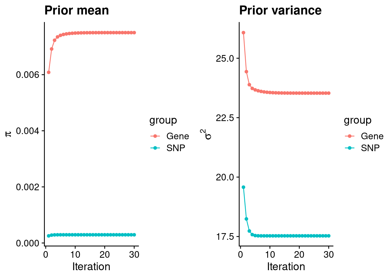
#estimated group prior
estimated_group_prior <- group_prior_rec[,ncol(group_prior_rec)]
names(estimated_group_prior) <- c("gene", "snp")
estimated_group_prior["snp"] <- estimated_group_prior["snp"]*thin #adjust parameter to account for thin argument
print(estimated_group_prior)
gene snp
0.0074990118 0.0002925305 #estimated group prior variance
estimated_group_prior_var <- group_prior_var_rec[,ncol(group_prior_var_rec)]
names(estimated_group_prior_var) <- c("gene", "snp")
print(estimated_group_prior_var) gene snp
23.53208 17.52845 #report sample size
print(sample_size)[1] 336107#report group size
group_size <- c(nrow(ctwas_gene_res), n_snps)
print(group_size)[1] 10973 7535010#estimated group PVE
estimated_group_pve <- estimated_group_prior_var*estimated_group_prior*group_size/sample_size #check PVE calculation
names(estimated_group_pve) <- c("gene", "snp")
print(estimated_group_pve) gene snp
0.005761189 0.114953178 #compare sum(PIP*mu2/sample_size) with above PVE calculation
c(sum(ctwas_gene_res$PVE),sum(ctwas_snp_res$PVE))[1] 0.2223438 18.6718962Genes with highest PIPs
#distribution of PIPs
hist(ctwas_gene_res$susie_pip, xlim=c(0,1), main="Distribution of Gene PIPs")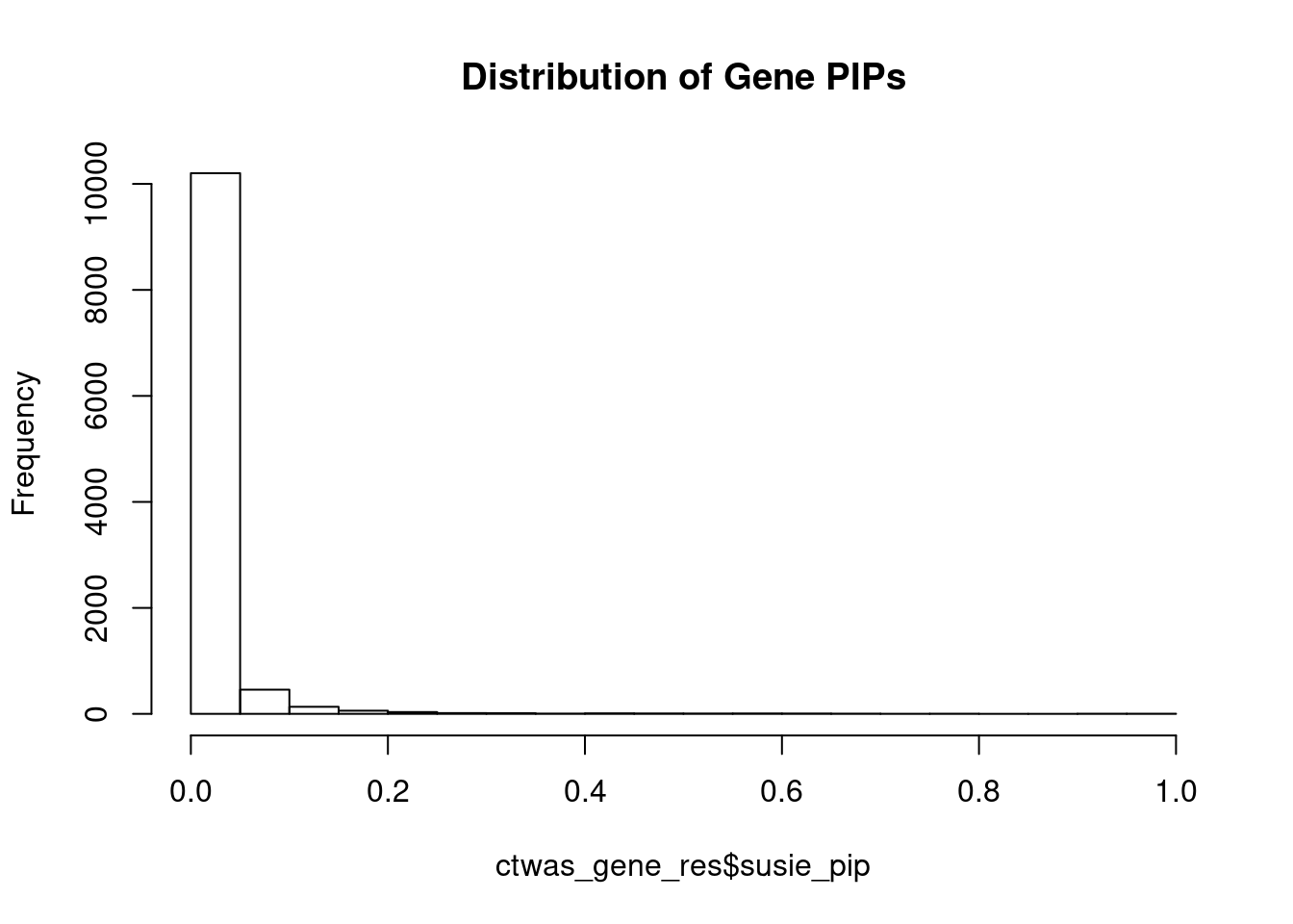
#genes with PIP>0.8 or 20 highest PIPs
head(ctwas_gene_res[order(-ctwas_gene_res$susie_pip),report_cols], max(sum(ctwas_gene_res$susie_pip>0.8), 20))
genename region_tag susie_pip mu2 PVE z
717 MAPK6 15_21 1.0000000 34111.65582 1.014905e-01 -4.600218
10029 GSAP 7_49 1.0000000 32344.91724 9.623399e-02 5.259703
7429 PPM1M 3_36 1.0000000 241.22300 7.176970e-04 4.468299
9989 ARL17A 17_27 0.9436863 32.40929 9.099544e-05 5.324914
1199 DYNLL1 12_74 0.9379920 59.07720 1.648699e-04 -5.805664
12053 ETV5 3_114 0.9122369 96.75415 2.626030e-04 9.862284
8671 EFEMP2 11_36 0.7914194 56.03230 1.319373e-04 -8.200649
3564 ZMIZ2 7_33 0.7782787 66.49342 1.539700e-04 -8.105339
9621 KCNB2 8_53 0.7522135 66.18833 1.481307e-04 -8.225507
13243 HIST1H2BE 6_20 0.7440818 31.09955 6.884892e-05 -6.515410
5796 ECE2 3_113 0.7149013 29.87117 6.353613e-05 -5.305115
1445 DERL3 22_6 0.6864450 22.98366 4.694047e-05 4.036538
7736 R3HCC1L 10_62 0.6829995 40.51919 8.233861e-05 7.438889
13421 PRICKLE4 6_32 0.6622145 24.65458 4.857567e-05 -4.797384
8923 ASPHD1 16_24 0.6555724 578.63592 1.128622e-03 -11.937656
11969 ATP5J2 7_61 0.6481907 53.45298 1.030854e-04 -7.116991
10750 UCKL1 20_38 0.6400369 25.30589 4.818913e-05 3.572515
151 CSDE1 1_71 0.6372136 22.68257 4.300311e-05 -4.744544
6243 DPYSL4 10_83 0.6345369 43.78509 8.266194e-05 -6.800654
9938 GPRIN3 4_60 0.6310406 25.08359 4.709442e-05 -3.768703
num_eqtl
717 1
10029 1
7429 2
9989 1
1199 1
12053 1
8671 1
3564 1
9621 1
13243 1
5796 1
1445 1
7736 1
13421 1
8923 1
11969 1
10750 1
151 1
6243 1
9938 2Genes with largest effect sizes
#plot PIP vs effect size
plot(ctwas_gene_res$susie_pip, ctwas_gene_res$mu2, xlab="PIP", ylab="mu^2", main="Gene PIPs vs Effect Size")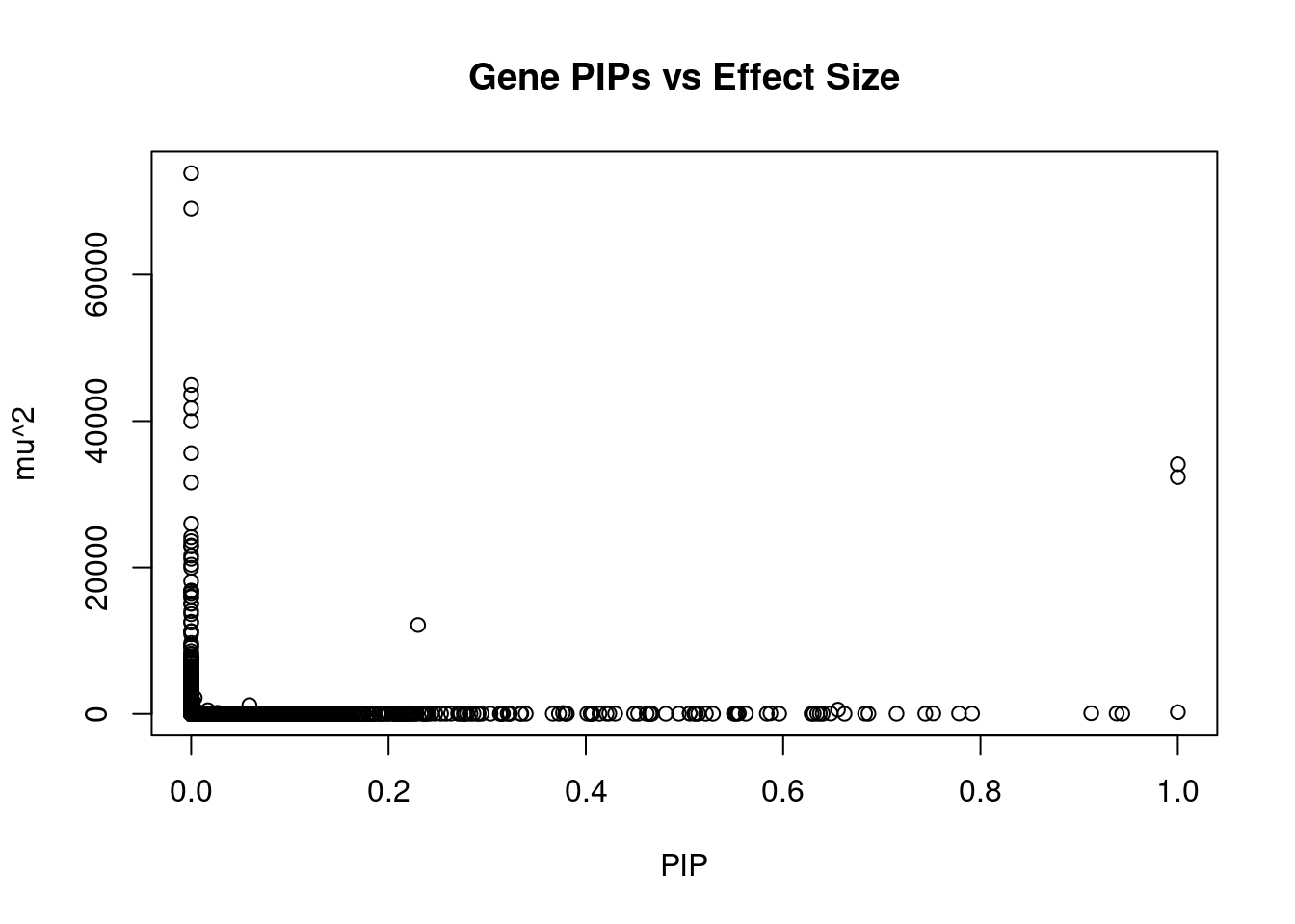
#genes with 20 largest effect sizes
head(ctwas_gene_res[order(-ctwas_gene_res$mu2),report_cols],20)
genename region_tag susie_pip mu2 PVE z
10 SEMA3F 3_35 0.000000e+00 73861.11 0.000000e+00 7.681163
10261 SLC38A3 3_35 0.000000e+00 69033.76 0.000000e+00 6.725828
7591 CCDC171 9_13 0.000000e+00 44932.09 0.000000e+00 7.405453
8624 NEGR1 1_46 0.000000e+00 43597.35 0.000000e+00 -10.374619
40 RBM6 3_35 0.000000e+00 41746.10 0.000000e+00 12.536042
6640 ZNF689 16_24 0.000000e+00 39994.39 0.000000e+00 -6.014416
7425 MST1R 3_35 0.000000e+00 35623.61 0.000000e+00 -12.634816
717 MAPK6 15_21 1.000000e+00 34111.66 1.014905e-01 -4.600218
10029 GSAP 7_49 1.000000e+00 32344.92 9.623399e-02 5.259703
9293 STX19 3_59 0.000000e+00 31600.11 0.000000e+00 -5.059656
9289 DHFR2 3_59 0.000000e+00 25976.41 0.000000e+00 4.031467
5274 MFAP1 15_16 1.202121e-06 24146.55 8.636263e-08 4.302998
7420 RNF123 3_35 0.000000e+00 23601.01 0.000000e+00 -10.959165
12024 NAT6 3_35 0.000000e+00 23005.37 0.000000e+00 -6.362236
10512 C6orf106 6_29 0.000000e+00 22878.38 0.000000e+00 2.961936
11433 CKMT1A 15_16 0.000000e+00 21624.66 0.000000e+00 4.129652
1326 WDR76 15_16 0.000000e+00 21190.22 0.000000e+00 4.963393
1785 ZNF629 16_24 0.000000e+00 20375.42 0.000000e+00 4.335360
10290 DPYD 1_60 0.000000e+00 19960.73 0.000000e+00 -3.213351
10101 HYAL3 3_35 0.000000e+00 18111.05 0.000000e+00 6.242668
num_eqtl
10 1
10261 1
7591 2
8624 2
40 1
6640 1
7425 2
717 1
10029 1
9293 1
9289 2
5274 1
7420 1
12024 1
10512 1
11433 1
1326 2
1785 1
10290 1
10101 2Genes with highest PVE
#genes with 20 highest pve
head(ctwas_gene_res[order(-ctwas_gene_res$PVE),report_cols],20)
genename region_tag susie_pip mu2 PVE z
717 MAPK6 15_21 1.00000000 34111.65582 1.014905e-01 -4.600218
10029 GSAP 7_49 1.00000000 32344.91724 9.623399e-02 5.259703
821 SDHA 5_1 0.22996475 12142.57236 8.307960e-03 2.906571
8923 ASPHD1 16_24 0.65557239 578.63592 1.128622e-03 -11.937656
7429 PPM1M 3_36 0.99999995 241.22300 7.176970e-04 4.468299
12053 ETV5 3_114 0.91223693 96.75415 2.626030e-04 9.862284
6834 ADPGK 15_34 0.05906579 1201.54605 2.111538e-04 5.872014
1199 DYNLL1 12_74 0.93799195 59.07720 1.648699e-04 -5.805664
3564 ZMIZ2 7_33 0.77827868 66.49342 1.539700e-04 -8.105339
9621 KCNB2 8_53 0.75221351 66.18833 1.481307e-04 -8.225507
6587 GPR61 1_67 0.58712009 79.87169 1.395219e-04 8.755235
5143 USO1 4_51 0.37686900 123.86534 1.388873e-04 -2.133639
8671 EFEMP2 11_36 0.79141941 56.03230 1.319373e-04 -8.200649
9035 NUPR1 16_23 0.55508807 69.66893 1.150598e-04 -10.643364
11969 ATP5J2 7_61 0.64819070 53.45298 1.030854e-04 -7.116991
10366 SLC35E2B 1_1 0.50528267 63.52597 9.550105e-05 -7.654473
12120 CDK11B 1_1 0.50528267 63.52597 9.550105e-05 -7.654473
9989 ARL17A 17_27 0.94368626 32.40929 9.099544e-05 5.324914
6243 DPYSL4 10_83 0.63453692 43.78509 8.266194e-05 -6.800654
7736 R3HCC1L 10_62 0.68299949 40.51919 8.233861e-05 7.438889
num_eqtl
717 1
10029 1
821 1
8923 1
7429 2
12053 1
6834 3
1199 1
3564 1
9621 1
6587 1
5143 1
8671 1
9035 2
11969 1
10366 1
12120 1
9989 1
6243 1
7736 1Genes with largest z scores
#genes with 20 largest z scores
head(ctwas_gene_res[order(-abs(ctwas_gene_res$z)),report_cols],20)
genename region_tag susie_pip mu2 PVE z
7425 MST1R 3_35 0.000000e+00 35623.60624 0.000000e+00 -12.634816
40 RBM6 3_35 0.000000e+00 41746.09899 0.000000e+00 12.536042
8923 ASPHD1 16_24 6.555724e-01 578.63592 1.128622e-03 -11.937656
8924 KCTD13 16_24 4.363856e-03 498.26763 6.469273e-06 11.490673
8275 INO80E 16_24 1.638102e-04 1631.74862 7.952738e-07 11.076716
7420 RNF123 3_35 0.000000e+00 23601.01392 0.000000e+00 -10.959165
6146 TAOK2 16_24 4.676057e-06 1891.49051 2.631518e-08 10.737701
9035 NUPR1 16_23 5.550881e-01 69.66893 1.150598e-04 -10.643364
8624 NEGR1 1_46 0.000000e+00 43597.35168 0.000000e+00 -10.374619
11727 RP11-196G11.6 16_24 4.163481e-08 7371.38703 9.131207e-10 10.011241
8623 C1QTNF4 11_29 2.296909e-02 95.37723 6.517949e-06 9.951168
12053 ETV5 3_114 9.122369e-01 96.75415 2.626030e-04 9.862284
5469 SAE1 19_33 4.553008e-03 100.30006 1.358695e-06 9.848747
461 PRSS8 16_24 2.774712e-09 6922.86884 5.715134e-11 -9.764760
7720 RAPSN 11_29 1.189135e-02 88.20982 3.120834e-06 9.728710
11241 LAT 16_23 2.439066e-01 56.17058 4.076195e-05 -9.552834
2491 MTCH2 11_29 9.481212e-03 83.09943 2.344144e-06 -9.514152
10579 IL27 16_23 6.175921e-03 50.93657 9.359526e-07 9.140265
3527 POLK 5_44 1.241711e-02 53.54319 1.978094e-06 8.883506
7718 SLC39A13 11_29 9.707601e-03 72.48101 2.093431e-06 -8.831101
num_eqtl
7425 2
40 1
8923 1
8924 1
8275 1
7420 1
6146 1
9035 2
8624 2
11727 1
8623 2
12053 1
5469 1
461 1
7720 1
11241 1
2491 1
10579 1
3527 1
7718 1Comparing z scores and PIPs
#set nominal signifiance threshold for z scores
alpha <- 0.05

#bonferroni adjusted threshold for z scores
sig_thresh <- qnorm(1-(alpha/nrow(ctwas_gene_res)/2), lower=T)

#Q-Q plot for z scores
obs_z <- ctwas_gene_res$z[order(ctwas_gene_res$z)]
exp_z <- qnorm((1:nrow(ctwas_gene_res))/nrow(ctwas_gene_res))

plot(exp_z, obs_z, xlab="Expected z", ylab="Observed z", main="Gene z score Q-Q plot")
abline(a=0,b=1)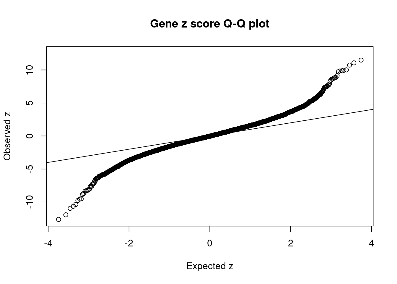
#plot z score vs PIP
plot(abs(ctwas_gene_res$z), ctwas_gene_res$susie_pip, xlab="abs(z)", ylab="PIP")
abline(v=sig_thresh, col="red", lty=2)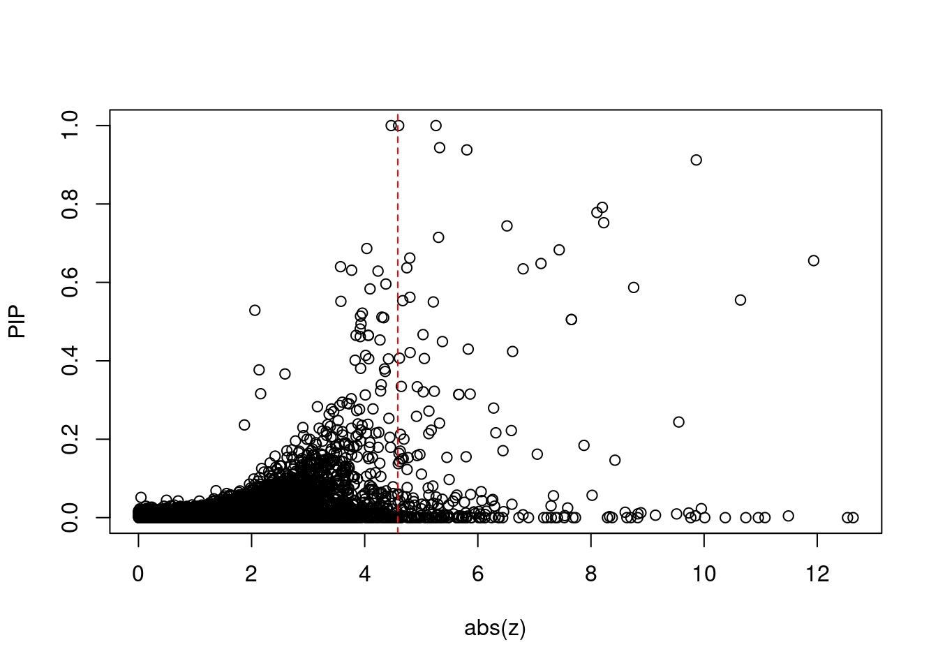
#proportion of significant z scores
mean(abs(ctwas_gene_res$z) > sig_thresh)
[1] 0.02159847#genes with most significant z scores
head(ctwas_gene_res[order(-abs(ctwas_gene_res$z)),report_cols],20) genename region_tag susie_pip mu2 PVE z
7425 MST1R 3_35 0.000000e+00 35623.60624 0.000000e+00 -12.634816
40 RBM6 3_35 0.000000e+00 41746.09899 0.000000e+00 12.536042
8923 ASPHD1 16_24 6.555724e-01 578.63592 1.128622e-03 -11.937656
8924 KCTD13 16_24 4.363856e-03 498.26763 6.469273e-06 11.490673
8275 INO80E 16_24 1.638102e-04 1631.74862 7.952738e-07 11.076716
7420 RNF123 3_35 0.000000e+00 23601.01392 0.000000e+00 -10.959165
6146 TAOK2 16_24 4.676057e-06 1891.49051 2.631518e-08 10.737701
9035 NUPR1 16_23 5.550881e-01 69.66893 1.150598e-04 -10.643364
8624 NEGR1 1_46 0.000000e+00 43597.35168 0.000000e+00 -10.374619
11727 RP11-196G11.6 16_24 4.163481e-08 7371.38703 9.131207e-10 10.011241
8623 C1QTNF4 11_29 2.296909e-02 95.37723 6.517949e-06 9.951168
12053 ETV5 3_114 9.122369e-01 96.75415 2.626030e-04 9.862284
5469 SAE1 19_33 4.553008e-03 100.30006 1.358695e-06 9.848747
461 PRSS8 16_24 2.774712e-09 6922.86884 5.715134e-11 -9.764760
7720 RAPSN 11_29 1.189135e-02 88.20982 3.120834e-06 9.728710
11241 LAT 16_23 2.439066e-01 56.17058 4.076195e-05 -9.552834
2491 MTCH2 11_29 9.481212e-03 83.09943 2.344144e-06 -9.514152
10579 IL27 16_23 6.175921e-03 50.93657 9.359526e-07 9.140265
3527 POLK 5_44 1.241711e-02 53.54319 1.978094e-06 8.883506
7718 SLC39A13 11_29 9.707601e-03 72.48101 2.093431e-06 -8.831101
num_eqtl
7425 2
40 1
8923 1
8924 1
8275 1
7420 1
6146 1
9035 2
8624 2
11727 1
8623 2
12053 1
5469 1
461 1
7720 1
11241 1
2491 1
10579 1
3527 1
7718 1Sensitivity, specificity and precision for silver standard genes
library("readxl")

known_annotations <- read_xlsx("data/summary_known_genes_annotations.xlsx", sheet="BMI")
known_annotations <- unique(known_annotations$`Gene Symbol`)

unrelated_genes <- ctwas_gene_res$genename[!(ctwas_gene_res$genename %in% known_annotations)]

#number of genes in known annotations
print(length(known_annotations))
[1] 41#number of genes in known annotations with imputed expression
print(sum(known_annotations %in% ctwas_gene_res$genename))[1] 25#assign ctwas, TWAS, and bystander genes
ctwas_genes <- ctwas_gene_res$genename[ctwas_gene_res$susie_pip>0.8]
twas_genes <- ctwas_gene_res$genename[abs(ctwas_gene_res$z)>sig_thresh]
novel_genes <- ctwas_genes[!(ctwas_genes %in% twas_genes)]
#significance threshold for TWAS
print(sig_thresh)[1] 4.584229#number of ctwas genes
length(ctwas_genes)[1] 6#number of TWAS genes
length(twas_genes)[1] 237#show novel genes (ctwas genes with not in TWAS genes)
ctwas_gene_res[ctwas_gene_res$genename %in% novel_genes,report_cols] genename region_tag susie_pip mu2 PVE z num_eqtl
7429 PPM1M 3_36 1 241.223 0.000717697 4.468299 2#sensitivity / recall
sensitivity <- rep(NA,2)
names(sensitivity) <- c("ctwas", "TWAS")
sensitivity["ctwas"] <- sum(ctwas_genes %in% known_annotations)/length(known_annotations)
sensitivity["TWAS"] <- sum(twas_genes %in% known_annotations)/length(known_annotations)
sensitivity ctwas TWAS
0.00000000 0.09756098 #specificity
specificity <- rep(NA,2)
names(specificity) <- c("ctwas", "TWAS")
specificity["ctwas"] <- sum(!(unrelated_genes %in% ctwas_genes))/length(unrelated_genes)
specificity["TWAS"] <- sum(!(unrelated_genes %in% twas_genes))/length(unrelated_genes)
specificity ctwas TWAS
0.9994520 0.9787176 #precision / PPV
precision <- rep(NA,2)
names(precision) <- c("ctwas", "TWAS")
precision["ctwas"] <- sum(ctwas_genes %in% known_annotations)/length(ctwas_genes)
precision["TWAS"] <- sum(twas_genes %in% known_annotations)/length(twas_genes)
precision ctwas TWAS
0.00000000 0.01687764 #ROC curves
pip_range <- (0:1000)/1000
sensitivity <- rep(NA, length(pip_range))
specificity <- rep(NA, length(pip_range))
for (index in 1:length(pip_range)){
pip <- pip_range[index]
ctwas_genes <- ctwas_gene_res$genename[ctwas_gene_res$susie_pip>=pip]
sensitivity[index] <- sum(ctwas_genes %in% known_annotations)/length(known_annotations)
specificity[index] <- sum(!(unrelated_genes %in% ctwas_genes))/length(unrelated_genes)
}
plot(1-specificity, sensitivity, type="l", xlim=c(0,1), ylim=c(0,1))
sig_thresh_range <- seq(from=0, to=max(abs(ctwas_gene_res$z)), length.out=length(pip_range))
for (index in 1:length(sig_thresh_range)){
sig_thresh_plot <- sig_thresh_range[index]
twas_genes <- ctwas_gene_res$genename[abs(ctwas_gene_res$z)>=sig_thresh_plot]
sensitivity[index] <- sum(twas_genes %in% known_annotations)/length(known_annotations)
specificity[index] <- sum(!(unrelated_genes %in% twas_genes))/length(unrelated_genes)
}
lines(1-specificity, sensitivity, xlim=c(0,1), ylim=c(0,1), col="red", lty=2)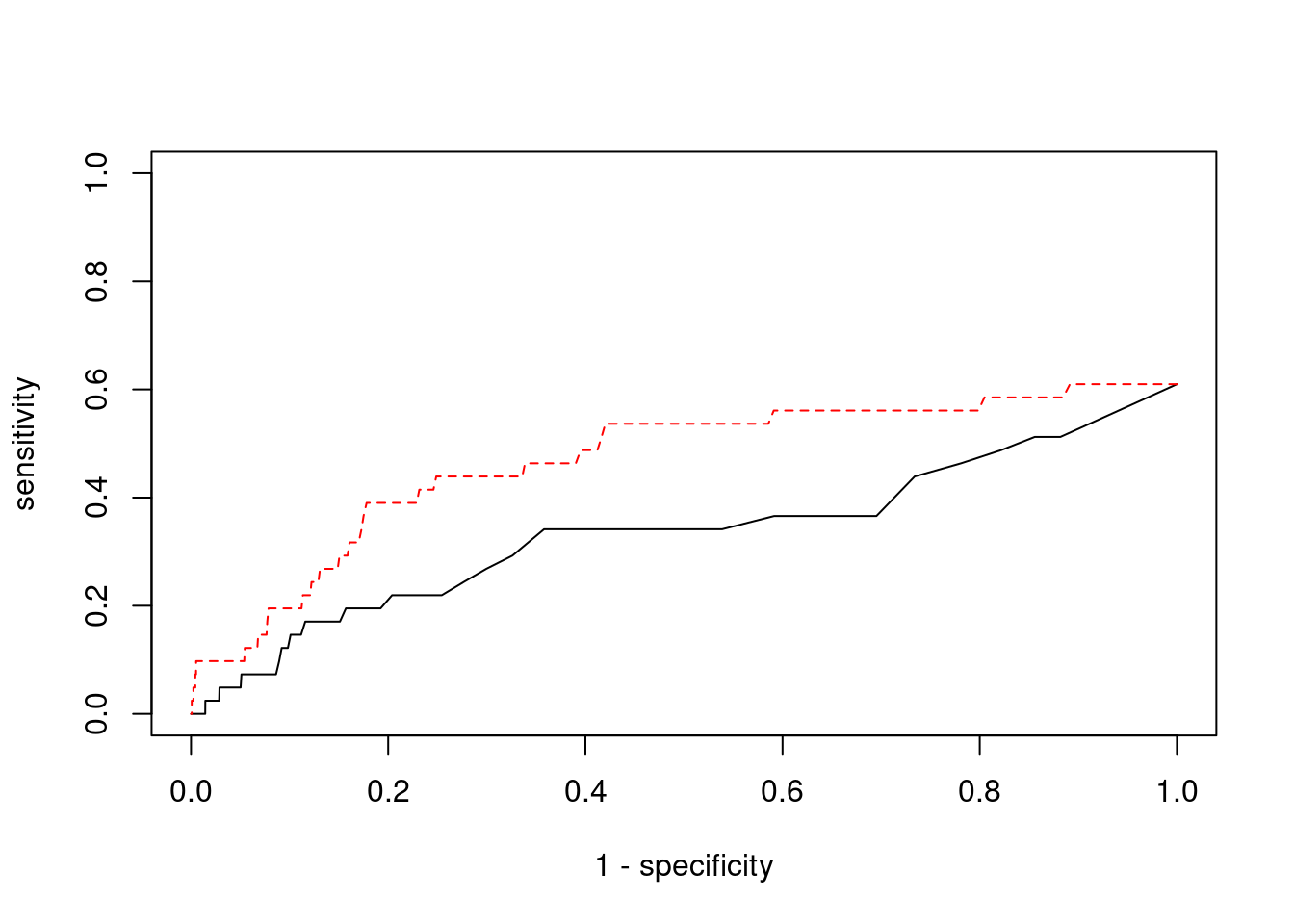
sessionInfo()R version 3.6.1 (2019-07-05)
Platform: x86_64-pc-linux-gnu (64-bit)
Running under: Scientific Linux 7.4 (Nitrogen)
Matrix products: default
BLAS/LAPACK: /software/openblas-0.2.19-el7-x86_64/lib/libopenblas_haswellp-r0.2.19.so
locale:
[1] LC_CTYPE=en_US.UTF-8 LC_NUMERIC=C
[3] LC_TIME=en_US.UTF-8 LC_COLLATE=en_US.UTF-8
[5] LC_MONETARY=en_US.UTF-8 LC_MESSAGES=en_US.UTF-8
[7] LC_PAPER=en_US.UTF-8 LC_NAME=C
[9] LC_ADDRESS=C LC_TELEPHONE=C
[11] LC_MEASUREMENT=en_US.UTF-8 LC_IDENTIFICATION=C
attached base packages:
[1] stats graphics grDevices utils datasets methods base
other attached packages:
[1] readxl_1.3.1 cowplot_1.0.0 ggplot2_3.3.5 workflowr_1.6.2
loaded via a namespace (and not attached):
[1] tidyselect_1.1.1 xfun_0.29 purrr_0.3.4 colorspace_2.0-2
[5] vctrs_0.3.8 generics_0.1.1 htmltools_0.5.2 yaml_2.2.1
[9] utf8_1.2.2 blob_1.2.2 rlang_0.4.12 jquerylib_0.1.4
[13] later_0.8.0 pillar_1.6.4 glue_1.5.1 withr_2.4.3
[17] DBI_1.1.1 bit64_4.0.5 lifecycle_1.0.1 stringr_1.4.0
[21] cellranger_1.1.0 munsell_0.5.0 gtable_0.3.0 evaluate_0.14
[25] memoise_2.0.1 labeling_0.4.2 knitr_1.36 fastmap_1.1.0
[29] httpuv_1.5.1 fansi_0.5.0 highr_0.9 Rcpp_1.0.7
[33] promises_1.0.1 scales_1.1.1 cachem_1.0.6 farver_2.1.0
[37] fs_1.5.2 bit_4.0.4 digest_0.6.29 stringi_1.7.6
[41] dplyr_1.0.7 rprojroot_2.0.2 grid_3.6.1 tools_3.6.1
[45] magrittr_2.0.1 tibble_3.1.6 RSQLite_2.2.8 crayon_1.4.2
[49] whisker_0.3-2 pkgconfig_2.0.3 ellipsis_0.3.2 data.table_1.14.2
[53] assertthat_0.2.1 rmarkdown_2.11 R6_2.5.1 git2r_0.26.1
[57] compiler_3.6.1