T2D - Adipose Subcutaneous
sheng Qian
2021-2-6
Last updated: 2022-02-13
Checks: 6 1
Knit directory: cTWAS_analysis/
This reproducible R Markdown analysis was created with workflowr (version 1.6.2). The Checks tab describes the reproducibility checks that were applied when the results were created. The Past versions tab lists the development history.
Great! Since the R Markdown file has been committed to the Git repository, you know the exact version of the code that produced these results.
Great job! The global environment was empty. Objects defined in the global environment can affect the analysis in your R Markdown file in unknown ways. For reproduciblity it’s best to always run the code in an empty environment.
The command set.seed(20211220) was run prior to running the code in the R Markdown file. Setting a seed ensures that any results that rely on randomness, e.g. subsampling or permutations, are reproducible.
Great job! Recording the operating system, R version, and package versions is critical for reproducibility.
Nice! There were no cached chunks for this analysis, so you can be confident that you successfully produced the results during this run.
Using absolute paths to the files within your workflowr project makes it difficult for you and others to run your code on a different machine. Change the absolute path(s) below to the suggested relative path(s) to make your code more reproducible.
| absolute | relative |
|---|---|
| /project2/xinhe/shengqian/cTWAS/cTWAS_analysis/data/ | data |
| /project2/xinhe/shengqian/cTWAS/cTWAS_analysis/code/ctwas_config.R | code/ctwas_config.R |
Great! You are using Git for version control. Tracking code development and connecting the code version to the results is critical for reproducibility.
The results in this page were generated with repository version 87fee8b. See the Past versions tab to see a history of the changes made to the R Markdown and HTML files.
Note that you need to be careful to ensure that all relevant files for the analysis have been committed to Git prior to generating the results (you can use wflow_publish or wflow_git_commit). workflowr only checks the R Markdown file, but you know if there are other scripts or data files that it depends on. Below is the status of the Git repository when the results were generated:
Ignored files:
    Ignored:    .ipynb_checkpoints/

Untracked files:
    Untracked:  code/.ipynb_checkpoints/
    Untracked:  code/AF_out/
    Untracked:  code/BMI_out/
    Untracked:  code/T2D_out/
    Untracked:  code/ctwas_config.R
    Untracked:  code/mapping.R
    Untracked:  code/out/
    Untracked:  code/run_AF_analysis.sbatch
    Untracked:  code/run_AF_analysis.sh
    Untracked:  code/run_AF_ctwas_rss_LDR.R
    Untracked:  code/run_BMI_analysis.sbatch
    Untracked:  code/run_BMI_analysis.sh
    Untracked:  code/run_BMI_ctwas_rss_LDR.R
    Untracked:  code/run_T2D_analysis.sbatch
    Untracked:  code/run_T2D_analysis.sh
    Untracked:  code/run_T2D_ctwas_rss_LDR.R
    Untracked:  data/.ipynb_checkpoints/
    Untracked:  data/AF/
    Untracked:  data/BMI/
    Untracked:  data/T2D/
    Untracked:  data/UKBB/
    Untracked:  data/UKBB_SNPs_Info.text
    Untracked:  data/gene_OMIM.txt
    Untracked:  data/gene_pip_0.8.txt
    Untracked:  data/mashr_Heart_Atrial_Appendage.db
    Untracked:  data/summary_known_genes_annotations.xlsx
    Untracked:  data/untitled.txt
Note that any generated files, e.g. HTML, png, CSS, etc., are not included in this status report because it is ok for generated content to have uncommitted changes.
These are the previous versions of the repository in which changes were made to the R Markdown (analysis/T2D_Adipose_Subcutaneous.Rmd) and HTML (docs/T2D_Adipose_Subcutaneous.html) files. If you’ve configured a remote Git repository (see ?wflow_git_remote), click on the hyperlinks in the table below to view the files as they were in that past version.
| File | Version | Author | Date | Message |
|---|---|---|---|---|
| Rmd | 87fee8b | sq-96 | 2022-02-13 | update |
Introduction
Weight QC
qclist_all <- list()

qc_files <- paste0(results_dir, "/", list.files(results_dir, pattern="exprqc.Rd"))

for (i in 1:length(qc_files)){
  load(qc_files[i])
  chr <- unlist(strsplit(rev(unlist(strsplit(qc_files[i], "_")))[1], "[.]"))[1]
  qclist_all[[chr]] <- cbind(do.call(rbind, lapply(qclist,unlist)), as.numeric(substring(chr,4)))
}

qclist_all <- data.frame(do.call(rbind, qclist_all))
colnames(qclist_all)[ncol(qclist_all)] <- "chr"

rm(qclist, wgtlist, z_gene_chr)

#number of imputed weights
nrow(qclist_all)
[1] 12414#number of imputed weights by chromosome
table(qclist_all$chr)
   1    2    3    4    5    6    7    8    9   10   11   12   13   14   15   16
1223  885  712  493  574  708  607  468  472  481  750  671  248  411  431  580
  17   18   19   20   21   22
 758  186  940  370  138  308
#number of imputed weights without missing variants
sum(qclist_all$nmiss==0)[1] 8861#proportion of imputed weights without missing variants
mean(qclist_all$nmiss==0)[1] 0.7137909Load ctwas results
Check convergence of parameters
library(ggplot2)
library(cowplot)
********************************************************Note: As of version 1.0.0, cowplot does not change the default ggplot2 theme anymore. To recover the previous behavior, execute:
theme_set(theme_cowplot())********************************************************load(paste0(results_dir, "/", analysis_id, "_ctwas.s2.susieIrssres.Rd"))
df <- data.frame(niter = rep(1:ncol(group_prior_rec), 2),
value = c(group_prior_rec[1,], group_prior_rec[2,]),
group = rep(c("Gene", "SNP"), each = ncol(group_prior_rec)))
df$group <- as.factor(df$group)
df$value[df$group=="SNP"] <- df$value[df$group=="SNP"]*thin #adjust parameter to account for thin argument
p_pi <- ggplot(df, aes(x=niter, y=value, group=group)) +
geom_line(aes(color=group)) +
geom_point(aes(color=group)) +
xlab("Iteration") + ylab(bquote(pi)) +
ggtitle("Prior mean") +
theme_cowplot()
df <- data.frame(niter = rep(1:ncol(group_prior_var_rec), 2),
value = c(group_prior_var_rec[1,], group_prior_var_rec[2,]),
group = rep(c("Gene", "SNP"), each = ncol(group_prior_var_rec)))
df$group <- as.factor(df$group)
p_sigma2 <- ggplot(df, aes(x=niter, y=value, group=group)) +
geom_line(aes(color=group)) +
geom_point(aes(color=group)) +
xlab("Iteration") + ylab(bquote(sigma^2)) +
ggtitle("Prior variance") +
theme_cowplot()
plot_grid(p_pi, p_sigma2)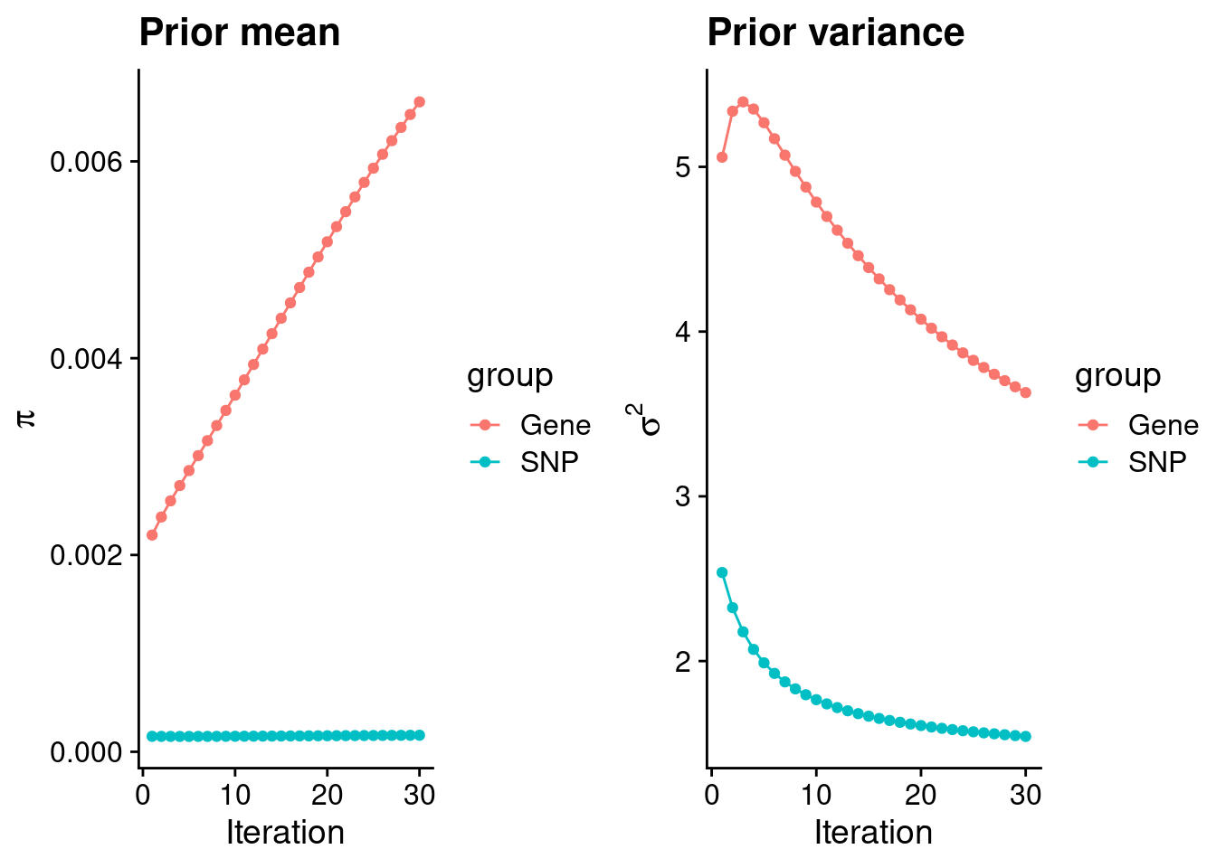
#estimated group prior
estimated_group_prior <- group_prior_rec[,ncol(group_prior_rec)]
names(estimated_group_prior) <- c("gene", "snp")
estimated_group_prior["snp"] <- estimated_group_prior["snp"]*thin #adjust parameter to account for thin argument
print(estimated_group_prior)
gene snp
0.0066047523 0.0001681642 #estimated group prior variance
estimated_group_prior_var <- group_prior_var_rec[,ncol(group_prior_var_rec)]
names(estimated_group_prior_var) <- c("gene", "snp")
print(estimated_group_prior_var) gene snp
3.629571 1.542519 #report sample size
print(sample_size)[1] 337159#report group size
group_size <- c(nrow(ctwas_gene_res), n_snps)
print(group_size)[1] 12414 7535010#estimated group PVE
estimated_group_pve <- estimated_group_prior_var*estimated_group_prior*group_size/sample_size #check PVE calculation
names(estimated_group_pve) <- c("gene", "snp")
print(estimated_group_pve) gene snp
0.0008826506 0.0057971306 #compare sum(PIP*mu2/sample_size) with above PVE calculation
c(sum(ctwas_gene_res$PVE),sum(ctwas_snp_res$PVE))[1] 0.008240852 0.104643058Genes with highest PIPs
#distribution of PIPs
hist(ctwas_gene_res$susie_pip, xlim=c(0,1), main="Distribution of Gene PIPs")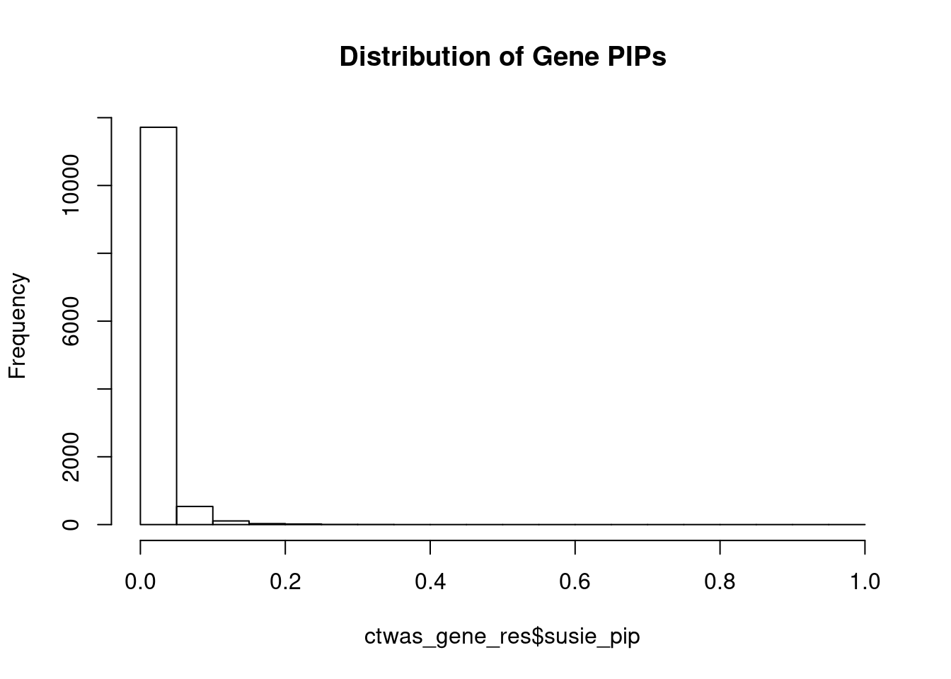
#genes with PIP>0.8 or 20 highest PIPs
head(ctwas_gene_res[order(-ctwas_gene_res$susie_pip),report_cols], max(sum(ctwas_gene_res$susie_pip>0.8), 20))
genename region_tag susie_pip mu2 PVE z num_eqtl
3633 CCND2 12_4 0.9960588 26.82338 7.924350e-05 5.640253 2
4039 DAW1 2_134 0.6520366 24.10133 4.660990e-05 4.212144 2
3927 KLHL7 7_20 0.3117293 28.82218 2.664831e-05 3.761454 2
1055 ADCY2 5_7 0.3110596 29.13539 2.688004e-05 -3.602686 1
5948 SAT2 17_7 0.3034725 27.90152 2.511380e-05 3.462292 1
8729 ZNF180 19_31 0.2994262 28.43816 2.525553e-05 3.487253 2
7067 NUS1 6_78 0.2961966 28.74758 2.525496e-05 3.716370 1
14507 RP6-65G23.5 14_33 0.2820679 26.95154 2.254771e-05 3.369949 1
2137 NIPAL2 8_67 0.2774893 29.77768 2.450769e-05 -3.500588 2
2923 GNPTAB 12_61 0.2585525 26.98745 2.069549e-05 3.600816 1
7368 AP3S2 15_41 0.2457994 26.57908 1.937697e-05 -3.675343 2
11538 RABL6 9_74 0.2439157 26.89396 1.945627e-05 -3.491221 1
8342 MAMDC2 9_31 0.2436855 27.46993 1.985420e-05 3.779388 1
7460 PINK1 1_14 0.2391013 26.38648 1.871237e-05 3.208561 1
5761 DIAPH3 13_28 0.2384631 26.45894 1.871366e-05 -3.353072 1
11408 RRP7A 22_18 0.2329284 25.57072 1.766569e-05 3.082913 4
7974 LMOD1 1_102 0.2310904 25.35682 1.737969e-05 3.200403 1
9603 HPSE 4_56 0.2282649 26.26893 1.778471e-05 -3.109502 1
10568 LIPF 10_56 0.2252638 26.18648 1.749580e-05 2.991710 1
12381 KCTD11 17_6 0.2232470 25.41206 1.682638e-05 3.070309 2Genes with largest effect sizes
#plot PIP vs effect size
plot(ctwas_gene_res$susie_pip, ctwas_gene_res$mu2, xlab="PIP", ylab="mu^2", main="Gene PIPs vs Effect Size")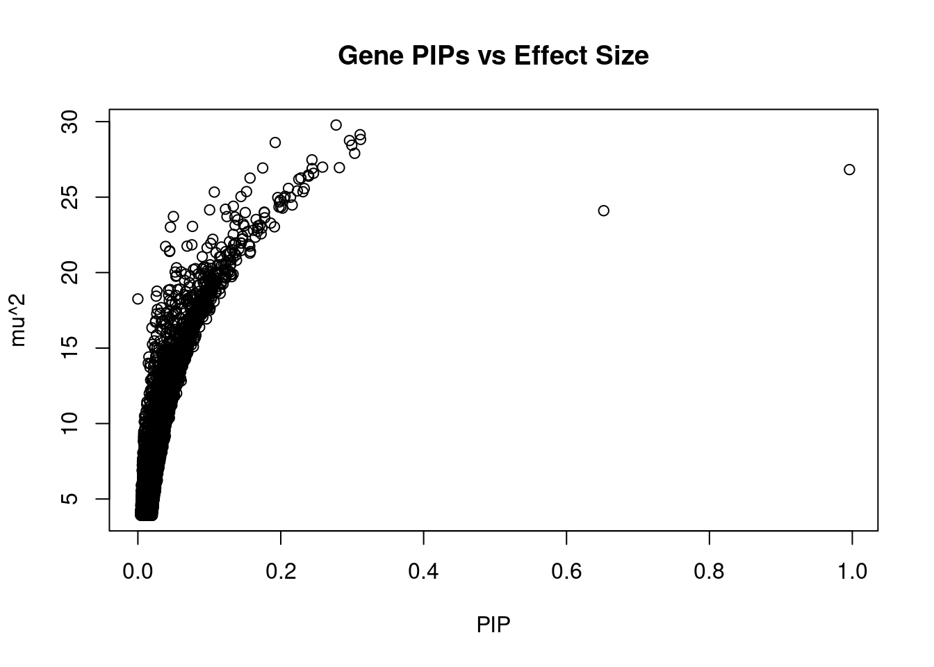
#genes with 20 largest effect sizes
head(ctwas_gene_res[order(-ctwas_gene_res$mu2),report_cols],20)
genename region_tag susie_pip mu2 PVE z num_eqtl
2137 NIPAL2 8_67 0.2774893 29.77768 2.450769e-05 -3.500588 2
1055 ADCY2 5_7 0.3110596 29.13539 2.688004e-05 -3.602686 1
3927 KLHL7 7_20 0.3117293 28.82218 2.664831e-05 3.761454 2
7067 NUS1 6_78 0.2961966 28.74758 2.525496e-05 3.716370 1
12700 LINC01537 11_41 0.1922338 28.61611 1.631569e-05 -3.271391 2
8729 ZNF180 19_31 0.2994262 28.43816 2.525553e-05 3.487253 2
5948 SAT2 17_7 0.3034725 27.90152 2.511380e-05 3.462292 1
8342 MAMDC2 9_31 0.2436855 27.46993 1.985420e-05 3.779388 1
2923 GNPTAB 12_61 0.2585525 26.98745 2.069549e-05 3.600816 1
14507 RP6-65G23.5 14_33 0.2820679 26.95154 2.254771e-05 3.369949 1
13511 AP001257.1 11_34 0.1747441 26.93090 1.395786e-05 3.363327 2
11538 RABL6 9_74 0.2439157 26.89396 1.945627e-05 -3.491221 1
3633 CCND2 12_4 0.9960588 26.82338 7.924350e-05 5.640253 2
7368 AP3S2 15_41 0.2457994 26.57908 1.937697e-05 -3.675343 2
5761 DIAPH3 13_28 0.2384631 26.45894 1.871366e-05 -3.353072 1
7460 PINK1 1_14 0.2391013 26.38648 1.871237e-05 3.208561 1
9603 HPSE 4_56 0.2282649 26.26893 1.778471e-05 -3.109502 1
12996 ZBED5 11_8 0.1569989 26.26162 1.222879e-05 -3.094448 2
10568 LIPF 10_56 0.2252638 26.18648 1.749580e-05 2.991710 1
9172 SIK2 11_66 0.2107616 25.57879 1.598957e-05 -3.728002 1Genes with highest PVE
#genes with 20 highest pve
head(ctwas_gene_res[order(-ctwas_gene_res$PVE),report_cols],20)
genename region_tag susie_pip mu2 PVE z num_eqtl
3633 CCND2 12_4 0.9960588 26.82338 7.924350e-05 5.640253 2
4039 DAW1 2_134 0.6520366 24.10133 4.660990e-05 4.212144 2
1055 ADCY2 5_7 0.3110596 29.13539 2.688004e-05 -3.602686 1
3927 KLHL7 7_20 0.3117293 28.82218 2.664831e-05 3.761454 2
8729 ZNF180 19_31 0.2994262 28.43816 2.525553e-05 3.487253 2
7067 NUS1 6_78 0.2961966 28.74758 2.525496e-05 3.716370 1
5948 SAT2 17_7 0.3034725 27.90152 2.511380e-05 3.462292 1
2137 NIPAL2 8_67 0.2774893 29.77768 2.450769e-05 -3.500588 2
14507 RP6-65G23.5 14_33 0.2820679 26.95154 2.254771e-05 3.369949 1
2923 GNPTAB 12_61 0.2585525 26.98745 2.069549e-05 3.600816 1
8342 MAMDC2 9_31 0.2436855 27.46993 1.985420e-05 3.779388 1
11538 RABL6 9_74 0.2439157 26.89396 1.945627e-05 -3.491221 1
7368 AP3S2 15_41 0.2457994 26.57908 1.937697e-05 -3.675343 2
5761 DIAPH3 13_28 0.2384631 26.45894 1.871366e-05 -3.353072 1
7460 PINK1 1_14 0.2391013 26.38648 1.871237e-05 3.208561 1
9603 HPSE 4_56 0.2282649 26.26893 1.778471e-05 -3.109502 1
11408 RRP7A 22_18 0.2329284 25.57072 1.766569e-05 3.082913 4
10568 LIPF 10_56 0.2252638 26.18648 1.749580e-05 2.991710 1
7974 LMOD1 1_102 0.2310904 25.35682 1.737969e-05 3.200403 1
12381 KCTD11 17_6 0.2232470 25.41206 1.682638e-05 3.070309 2Genes with largest z scores
#genes with 20 largest z scores
head(ctwas_gene_res[order(-abs(ctwas_gene_res$z)),report_cols],20)
genename region_tag susie_pip mu2 PVE z num_eqtl
3633 CCND2 12_4 0.99605876 26.82338 7.924350e-05 5.640253 2
4039 DAW1 2_134 0.65203660 24.10133 4.660990e-05 4.212144 2
8342 MAMDC2 9_31 0.24368551 27.46993 1.985420e-05 3.779388 1
3927 KLHL7 7_20 0.31172926 28.82218 2.664831e-05 3.761454 2
9172 SIK2 11_66 0.21076159 25.57879 1.598957e-05 -3.728002 1
7067 NUS1 6_78 0.29619664 28.74758 2.525496e-05 3.716370 1
7368 AP3S2 15_41 0.24579938 26.57908 1.937697e-05 -3.675343 2
1055 ADCY2 5_7 0.31105965 29.13539 2.688004e-05 -3.602686 1
2923 GNPTAB 12_61 0.25855245 26.98745 2.069549e-05 3.600816 1
6954 ZFP36L2 2_27 0.09181774 19.66710 5.355897e-06 -3.577139 2
1731 RBX1 22_17 0.17255431 22.56815 1.155013e-05 -3.521311 1
14659 LINC01126 2_27 0.08675796 19.20577 4.942040e-06 3.518883 2
2137 NIPAL2 8_67 0.27748935 29.77768 2.450769e-05 -3.500588 2
11538 RABL6 9_74 0.24391565 26.89396 1.945627e-05 -3.491221 1
8729 ZNF180 19_31 0.29942623 28.43816 2.525553e-05 3.487253 2
8071 SPDYA 2_17 0.13662530 21.97074 8.903094e-06 -3.478973 2
5948 SAT2 17_7 0.30347254 27.90152 2.511380e-05 3.462292 1
9512 DNAJB7 22_17 0.15659375 21.74971 1.010167e-05 3.462008 1
5651 CNOT6L 4_52 0.20603518 25.05407 1.531034e-05 3.460483 1
12362 PPP1CB 2_17 0.12457721 21.20505 7.835074e-06 3.405525 1Comparing z scores and PIPs
#set nominal signifiance threshold for z scores
alpha <- 0.05

#bonferroni adjusted threshold for z scores
sig_thresh <- qnorm(1-(alpha/nrow(ctwas_gene_res)/2), lower=T)

#Q-Q plot for z scores
obs_z <- ctwas_gene_res$z[order(ctwas_gene_res$z)]
exp_z <- qnorm((1:nrow(ctwas_gene_res))/nrow(ctwas_gene_res))

plot(exp_z, obs_z, xlab="Expected z", ylab="Observed z", main="Gene z score Q-Q plot")
abline(a=0,b=1)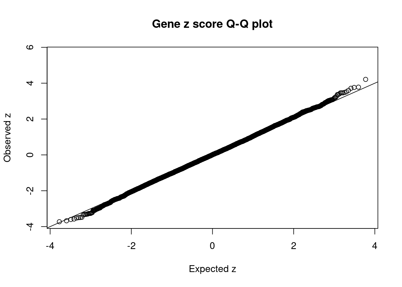
#plot z score vs PIP
plot(abs(ctwas_gene_res$z), ctwas_gene_res$susie_pip, xlab="abs(z)", ylab="PIP")
abline(v=sig_thresh, col="red", lty=2)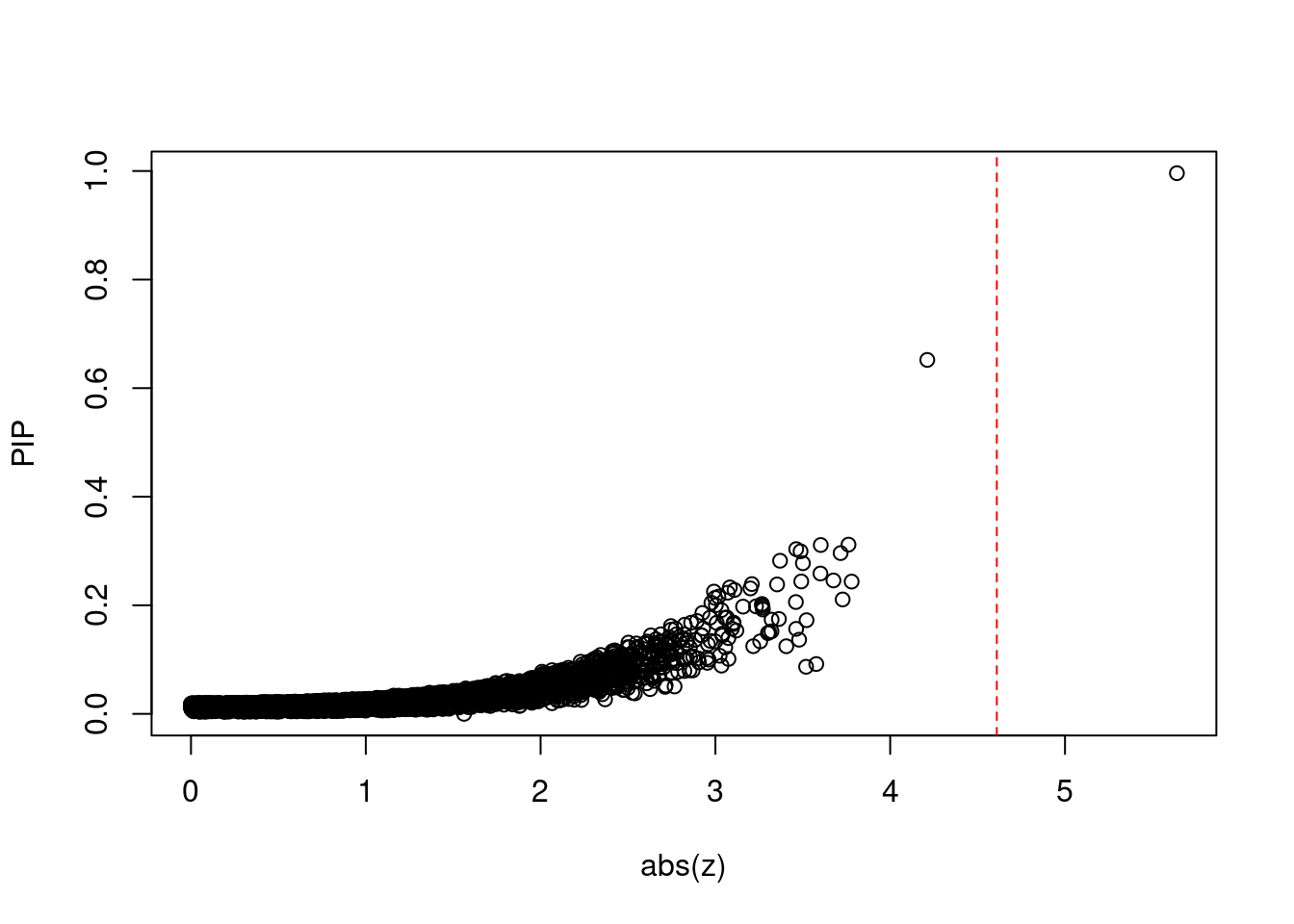
#proportion of significant z scores
mean(abs(ctwas_gene_res$z) > sig_thresh)
[1] 8.055421e-05#genes with most significant z scores
head(ctwas_gene_res[order(-abs(ctwas_gene_res$z)),report_cols],20) genename region_tag susie_pip mu2 PVE z num_eqtl
3633 CCND2 12_4 0.99605876 26.82338 7.924350e-05 5.640253 2
4039 DAW1 2_134 0.65203660 24.10133 4.660990e-05 4.212144 2
8342 MAMDC2 9_31 0.24368551 27.46993 1.985420e-05 3.779388 1
3927 KLHL7 7_20 0.31172926 28.82218 2.664831e-05 3.761454 2
9172 SIK2 11_66 0.21076159 25.57879 1.598957e-05 -3.728002 1
7067 NUS1 6_78 0.29619664 28.74758 2.525496e-05 3.716370 1
7368 AP3S2 15_41 0.24579938 26.57908 1.937697e-05 -3.675343 2
1055 ADCY2 5_7 0.31105965 29.13539 2.688004e-05 -3.602686 1
2923 GNPTAB 12_61 0.25855245 26.98745 2.069549e-05 3.600816 1
6954 ZFP36L2 2_27 0.09181774 19.66710 5.355897e-06 -3.577139 2
1731 RBX1 22_17 0.17255431 22.56815 1.155013e-05 -3.521311 1
14659 LINC01126 2_27 0.08675796 19.20577 4.942040e-06 3.518883 2
2137 NIPAL2 8_67 0.27748935 29.77768 2.450769e-05 -3.500588 2
11538 RABL6 9_74 0.24391565 26.89396 1.945627e-05 -3.491221 1
8729 ZNF180 19_31 0.29942623 28.43816 2.525553e-05 3.487253 2
8071 SPDYA 2_17 0.13662530 21.97074 8.903094e-06 -3.478973 2
5948 SAT2 17_7 0.30347254 27.90152 2.511380e-05 3.462292 1
9512 DNAJB7 22_17 0.15659375 21.74971 1.010167e-05 3.462008 1
5651 CNOT6L 4_52 0.20603518 25.05407 1.531034e-05 3.460483 1
12362 PPP1CB 2_17 0.12457721 21.20505 7.835074e-06 3.405525 1Sensitivity, specificity and precision for silver standard genes
library("readxl")

known_annotations <- read_xlsx("data/summary_known_genes_annotations.xlsx", sheet="T2D")
known_annotations <- unique(known_annotations$`Gene Symbol`)

unrelated_genes <- ctwas_gene_res$genename[!(ctwas_gene_res$genename %in% known_annotations)]

#number of genes in known annotations
print(length(known_annotations))
[1] 72#number of genes in known annotations with imputed expression
print(sum(known_annotations %in% ctwas_gene_res$genename))[1] 35#assign ctwas, TWAS, and bystander genes
ctwas_genes <- ctwas_gene_res$genename[ctwas_gene_res$susie_pip>0.8]
twas_genes <- ctwas_gene_res$genename[abs(ctwas_gene_res$z)>sig_thresh]
novel_genes <- ctwas_genes[!(ctwas_genes %in% twas_genes)]
#significance threshold for TWAS
print(sig_thresh)[1] 4.609947#number of ctwas genes
length(ctwas_genes)[1] 1#number of TWAS genes
length(twas_genes)[1] 1#show novel genes (ctwas genes with not in TWAS genes)
ctwas_gene_res[ctwas_gene_res$genename %in% novel_genes,report_cols][1] genename region_tag susie_pip mu2 PVE z num_eqtl
<0 rows> (or 0-length row.names)#sensitivity / recall
sensitivity <- rep(NA,2)
names(sensitivity) <- c("ctwas", "TWAS")
sensitivity["ctwas"] <- sum(ctwas_genes %in% known_annotations)/length(known_annotations)
sensitivity["TWAS"] <- sum(twas_genes %in% known_annotations)/length(known_annotations)
sensitivityctwas TWAS
0 0 #specificity
specificity <- rep(NA,2)
names(specificity) <- c("ctwas", "TWAS")
specificity["ctwas"] <- sum(!(unrelated_genes %in% ctwas_genes))/length(unrelated_genes)
specificity["TWAS"] <- sum(!(unrelated_genes %in% twas_genes))/length(unrelated_genes)
specificity ctwas TWAS
0.9999192 0.9999192 #precision / PPV
precision <- rep(NA,2)
names(precision) <- c("ctwas", "TWAS")
precision["ctwas"] <- sum(ctwas_genes %in% known_annotations)/length(ctwas_genes)
precision["TWAS"] <- sum(twas_genes %in% known_annotations)/length(twas_genes)
precisionctwas TWAS
0 0 #ROC curves
pip_range <- (0:1000)/1000
sensitivity <- rep(NA, length(pip_range))
specificity <- rep(NA, length(pip_range))
for (index in 1:length(pip_range)){
pip <- pip_range[index]
ctwas_genes <- ctwas_gene_res$genename[ctwas_gene_res$susie_pip>=pip]
sensitivity[index] <- sum(ctwas_genes %in% known_annotations)/length(known_annotations)
specificity[index] <- sum(!(unrelated_genes %in% ctwas_genes))/length(unrelated_genes)
}
plot(1-specificity, sensitivity, type="l", xlim=c(0,1), ylim=c(0,1))
sig_thresh_range <- seq(from=0, to=max(abs(ctwas_gene_res$z)), length.out=length(pip_range))
for (index in 1:length(sig_thresh_range)){
sig_thresh_plot <- sig_thresh_range[index]
twas_genes <- ctwas_gene_res$genename[abs(ctwas_gene_res$z)>=sig_thresh_plot]
sensitivity[index] <- sum(twas_genes %in% known_annotations)/length(known_annotations)
specificity[index] <- sum(!(unrelated_genes %in% twas_genes))/length(unrelated_genes)
}
lines(1-specificity, sensitivity, xlim=c(0,1), ylim=c(0,1), col="red", lty=2)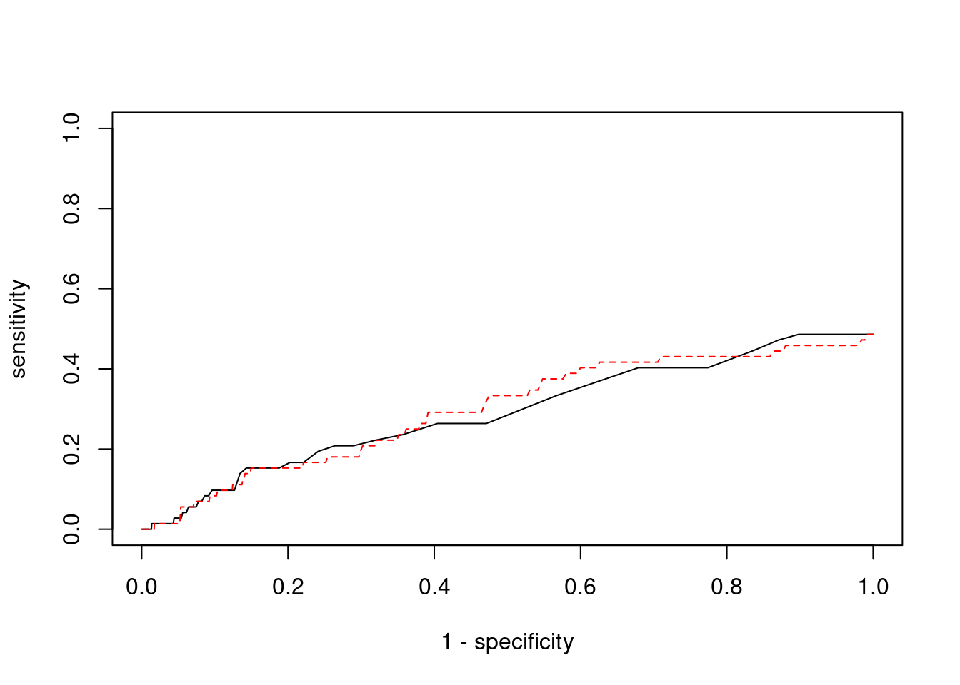
Sensitivity, specificity and precision for silver standard genes - bystanders only
This section first uses all silver standard genes to identify bystander genes within 1Mb. The silver standard and bystander gene lists are then subset to only genes with imputed expression in this analysis. Then, the ctwas and TWAS gene lists from this analysis are subset to only genes that are in the (subset) silver standard and bystander genes. These gene lists are then used to compute sensitivity, specificity and precision for ctwas and TWAS.
library(biomaRt)
library(GenomicRanges)Loading required package: stats4Loading required package: BiocGenericsLoading required package: parallel
Attaching package: 'BiocGenerics'The following objects are masked from 'package:parallel':
clusterApply, clusterApplyLB, clusterCall, clusterEvalQ,
clusterExport, clusterMap, parApply, parCapply, parLapply,
parLapplyLB, parRapply, parSapply, parSapplyLBThe following objects are masked from 'package:stats':
IQR, mad, sd, var, xtabsThe following objects are masked from 'package:base':
anyDuplicated, append, as.data.frame, basename, cbind, colnames,
dirname, do.call, duplicated, eval, evalq, Filter, Find, get, grep,
grepl, intersect, is.unsorted, lapply, Map, mapply, match, mget,
order, paste, pmax, pmax.int, pmin, pmin.int, Position, rank,
rbind, Reduce, rownames, sapply, setdiff, sort, table, tapply,
union, unique, unsplit, which, which.max, which.minLoading required package: S4Vectors
Attaching package: 'S4Vectors'The following object is masked from 'package:base':
expand.gridLoading required package: IRangesLoading required package: GenomeInfoDbensembl <- useEnsembl(biomart="ENSEMBL_MART_ENSEMBL", dataset="hsapiens_gene_ensembl")
G_list <- getBM(filters= "chromosome_name", attributes= c("hgnc_symbol","chromosome_name","start_position","end_position","gene_biotype"), values=1:22, mart=ensembl)
G_list <- G_list[G_list$hgnc_symbol!="",]
G_list <- G_list[G_list$gene_biotype %in% c("protein_coding","lncRNA"),]
G_list$start <- G_list$start_position
G_list$end <- G_list$end_position
G_list_granges <- makeGRangesFromDataFrame(G_list, keep.extra.columns=T)
known_annotations_positions <- G_list[G_list$hgnc_symbol %in% known_annotations,]
half_window <- 1000000
known_annotations_positions$start <- known_annotations_positions$start_position - half_window
known_annotations_positions$end <- known_annotations_positions$end_position + half_window
known_annotations_positions$start[known_annotations_positions$start<1] <- 1
known_annotations_granges <- makeGRangesFromDataFrame(known_annotations_positions, keep.extra.columns=T)
bystanders <- findOverlaps(known_annotations_granges,G_list_granges)
bystanders <- unique(subjectHits(bystanders))
bystanders <- G_list$hgnc_symbol[bystanders]
bystanders <- bystanders[!(bystanders %in% known_annotations)]
unrelated_genes <- bystanders
#number of genes in known annotations
print(length(known_annotations))[1] 72#number of genes in known annotations with imputed expression
print(sum(known_annotations %in% ctwas_gene_res$genename))[1] 35#number of bystander genes
print(length(unrelated_genes))[1] 1847#number of bystander genes with imputed expression
print(sum(unrelated_genes %in% ctwas_gene_res$genename))[1] 941#remove genes without imputed expression from gene lists
known_annotations <- known_annotations[known_annotations %in% ctwas_gene_res$genename]
unrelated_genes <- unrelated_genes[unrelated_genes %in% ctwas_gene_res$genename]
#assign ctwas and TWAS genes
ctwas_genes <- ctwas_gene_res$genename[ctwas_gene_res$susie_pip>0.8]
twas_genes <- ctwas_gene_res$genename[abs(ctwas_gene_res$z)>sig_thresh]
#significance threshold for TWAS
print(sig_thresh)[1] 4.609947#number of ctwas genes
length(ctwas_genes)[1] 1#number of ctwas genes in known annotations or bystanders
sum(ctwas_genes %in% c(known_annotations, unrelated_genes))[1] 0#number of ctwas genes
length(twas_genes)[1] 1#number of TWAS genes
sum(twas_genes %in% c(known_annotations, unrelated_genes))[1] 0#remove genes not in known or bystander lists from results
ctwas_genes <- ctwas_genes[ctwas_genes %in% c(known_annotations, unrelated_genes)]
twas_genes <- twas_genes[twas_genes %in% c(known_annotations, unrelated_genes)]
#sensitivity / recall
sensitivity <- rep(NA,2)
names(sensitivity) <- c("ctwas", "TWAS")
sensitivity["ctwas"] <- sum(ctwas_genes %in% known_annotations)/length(known_annotations)
sensitivity["TWAS"] <- sum(twas_genes %in% known_annotations)/length(known_annotations)
sensitivity
ctwas TWAS
0 0 #specificity
specificity <- rep(NA,2)
names(specificity) <- c("ctwas", "TWAS")
specificity["ctwas"] <- sum(!(unrelated_genes %in% ctwas_genes))/length(unrelated_genes)
specificity["TWAS"] <- sum(!(unrelated_genes %in% twas_genes))/length(unrelated_genes)
specificityctwas TWAS
1 1 #precision / PPV
precision <- rep(NA,2)
names(precision) <- c("ctwas", "TWAS")
precision["ctwas"] <- sum(ctwas_genes %in% known_annotations)/length(ctwas_genes)
precision["TWAS"] <- sum(twas_genes %in% known_annotations)/length(twas_genes)
precisionctwas TWAS
NaN NaN
sessionInfo()R version 3.6.1 (2019-07-05)
Platform: x86_64-pc-linux-gnu (64-bit)
Running under: Scientific Linux 7.4 (Nitrogen)
Matrix products: default
BLAS/LAPACK: /software/openblas-0.2.19-el7-x86_64/lib/libopenblas_haswellp-r0.2.19.so
locale:
[1] LC_CTYPE=en_US.UTF-8 LC_NUMERIC=C
[3] LC_TIME=en_US.UTF-8 LC_COLLATE=en_US.UTF-8
[5] LC_MONETARY=en_US.UTF-8 LC_MESSAGES=en_US.UTF-8
[7] LC_PAPER=en_US.UTF-8 LC_NAME=C
[9] LC_ADDRESS=C LC_TELEPHONE=C
[11] LC_MEASUREMENT=en_US.UTF-8 LC_IDENTIFICATION=C
attached base packages:
[1] parallel stats4 stats graphics grDevices utils datasets
[8] methods base
other attached packages:
[1] GenomicRanges_1.36.1 GenomeInfoDb_1.20.0 IRanges_2.18.1
[4] S4Vectors_0.22.1 BiocGenerics_0.30.0 biomaRt_2.40.1
[7] readxl_1.3.1 cowplot_1.0.0 ggplot2_3.3.5
[10] workflowr_1.6.2
loaded via a namespace (and not attached):
[1] Rcpp_1.0.7 prettyunits_1.1.1 assertthat_0.2.1
[4] rprojroot_2.0.2 digest_0.6.29 utf8_1.2.2
[7] R6_2.5.1 cellranger_1.1.0 RSQLite_2.2.8
[10] evaluate_0.14 httr_1.4.2 highr_0.9
[13] pillar_1.6.4 zlibbioc_1.30.0 progress_1.2.2
[16] rlang_0.4.12 curl_4.3.2 data.table_1.14.2
[19] whisker_0.3-2 jquerylib_0.1.4 blob_1.2.2
[22] rmarkdown_2.11 labeling_0.4.2 stringr_1.4.0
[25] RCurl_1.98-1.5 bit_4.0.4 munsell_0.5.0
[28] compiler_3.6.1 httpuv_1.5.1 xfun_0.29
[31] pkgconfig_2.0.3 htmltools_0.5.2 tidyselect_1.1.1
[34] GenomeInfoDbData_1.2.1 tibble_3.1.6 XML_3.99-0.3
[37] fansi_0.5.0 crayon_1.4.2 dplyr_1.0.7
[40] withr_2.4.3 later_0.8.0 bitops_1.0-7
[43] grid_3.6.1 gtable_0.3.0 lifecycle_1.0.1
[46] DBI_1.1.1 git2r_0.26.1 magrittr_2.0.1
[49] scales_1.1.1 stringi_1.7.6 cachem_1.0.6
[52] XVector_0.24.0 farver_2.1.0 fs_1.5.2
[55] promises_1.0.1 ellipsis_0.3.2 generics_0.1.1
[58] vctrs_0.3.8 tools_3.6.1 bit64_4.0.5
[61] Biobase_2.44.0 glue_1.5.1 purrr_0.3.4
[64] hms_1.1.1 fastmap_1.1.0 yaml_2.2.1
[67] AnnotationDbi_1.46.0 colorspace_2.0-2 memoise_2.0.1
[70] knitr_1.36