Enrichment analysis for 6 Traits, 5 tissues, eQTL + sQTL + stQTL – compute ukbb LD, eqtl, sqtl from predictdb; stQTL from Munro et al
XSun
2024-10-23
Last updated: 2024-10-29
Checks: 6 1
Knit directory: multigroup_ctwas_analysis/
This reproducible R Markdown analysis was created with workflowr (version 1.7.0). The Checks tab describes the reproducibility checks that were applied when the results were created. The Past versions tab lists the development history.
The R Markdown file has unstaged changes. To know which version of
the R Markdown file created these results, you’ll want to first commit
it to the Git repo. If you’re still working on the analysis, you can
ignore this warning. When you’re finished, you can run
wflow_publish to commit the R Markdown file and build the
HTML.
Great job! The global environment was empty. Objects defined in the global environment can affect the analysis in your R Markdown file in unknown ways. For reproduciblity it’s best to always run the code in an empty environment.
The command set.seed(20231112) was run prior to running
the code in the R Markdown file. Setting a seed ensures that any results
that rely on randomness, e.g. subsampling or permutations, are
reproducible.
Great job! Recording the operating system, R version, and package versions is critical for reproducibility.
Nice! There were no cached chunks for this analysis, so you can be confident that you successfully produced the results during this run.
Great job! Using relative paths to the files within your workflowr project makes it easier to run your code on other machines.
Great! You are using Git for version control. Tracking code development and connecting the code version to the results is critical for reproducibility.
The results in this page were generated with repository version 67b91ff. See the Past versions tab to see a history of the changes made to the R Markdown and HTML files.
Note that you need to be careful to ensure that all relevant files for
the analysis have been committed to Git prior to generating the results
(you can use wflow_publish or
wflow_git_commit). workflowr only checks the R Markdown
file, but you know if there are other scripts or data files that it
depends on. Below is the status of the Git repository when the results
were generated:
Ignored files:
    Ignored:    .Rhistory

Unstaged changes:
    Modified:   analysis/multi_group_6traits_15weights_ess_enrichment_genesymbol.Rmd
Note that any generated files, e.g. HTML, png, CSS, etc., are not included in this status report because it is ok for generated content to have uncommitted changes.
These are the previous versions of the repository in which changes were
made to the R Markdown
(analysis/multi_group_6traits_15weights_ess_enrichment_genesymbol.Rmd)
and HTML
(docs/multi_group_6traits_15weights_ess_enrichment_genesymbol.html)
files. If you’ve configured a remote Git repository (see
?wflow_git_remote), click on the hyperlinks in the table
below to view the files as they were in that past version.
| File | Version | Author | Date | Message |
|---|---|---|---|---|
| Rmd | ba30ddd | XSun | 2024-10-24 | update |
| html | ba30ddd | XSun | 2024-10-24 | update |
| Rmd | 2446887 | XSun | 2024-10-23 | update |
| html | 2446887 | XSun | 2024-10-23 | update |
 library(tidyr)
 library(dplyr)
 library(VennDiagram)
 library(ggplot2)

traits <- c("LDL-ukb-d-30780_irnt","SBP-ukb-a-360","WBC-ieu-b-30","aFib-ebi-a-GCST006414","SCZ-ieu-b-5102","IBD-ebi-a-GCST004131")
dbs <- c("GO_Biological_Process_2023","GO_Cellular_Component_2023","GO_Molecular_Function_2023")

# trait<- "LDL-ukb-d-30780_irnt"
# db <- "GO_Biological_Process_2023"

pval_threshold <- 0.001
Methods
We do enrichment analysis for the genes with PIP > 0.8 here: https://sq-96.github.io/multigroup_ctwas_analysis/multi_group_6traits_15weights_ess.html
The gene set membership was downloaded here: https://maayanlab.cloud/Enrichr/#libraries
Background genes
For Fractional model and Fisher exact test, we selected 2 kind of backgroud genes
- All genes used in ctwas
- All genes in the selected geneset database.
For enrichR, the background genes are not modifiable. The background genes are all genes in the selected geneset database
Using EnrichR package.
This package was used in our earlier ctwas paper.
- It takes a list of genes(genes with PIP > 0.8) as input and returns the enriched GO terms with adjusted p-values.
Fractional model
Model
The model is:
glm(PIP ~ gene set membership, family = quasibinomial('log10it')).
We do this regression for one gene set at a time.
The PIP vector contains:
- all genes within the credible set: we use their actual PIPs
- genes without the credible set & PIP < 0.1: we set the PIPs
as
0.5*min(gene pip within credible set)
The 2 different baselines:
- All genes from ctwas. Here,
genes without the credible set & PIP < 0.1includes only the genes used in ctwas. - All genes from the geneset database. Here,
genes without the credible set & PIP < 0.1includes the union of all genes from the GO terms in the geneset database.
p-value calibration
We used permutation testing to assess the
significance of associations between combined_pip and GO
terms. Permutation testing creates a “null” distribution by shuffling
data and recalculating p-values.
Initial log10istic Regression: For each GO term, a log10istic regression is performed using
glm(PIP ~ gene set membership, family = quasibinomial('log10it')). The observed p-value (pval_origin) measures the association strength in the actual data.Null Distributions via Permutation:
- Then we simulate random associations by shuffling the GO term
membership (
x) multiple times and recalculating the log10istic regression p-value for each shuffle. - These shuffled p-values represent what would be expected if there were no real association and create a “null” distribution.
- Then we simulate random associations by shuffling the GO term
membership (
Calibrated p-values with Increasing Permutations:
- The initial permutation test uses 1,000 shuffles
(
n_permutations = 1000) to compute a calibrated p-value (pval_calibrated), comparing the observed p-value against the null distribution. - Further Calibration: If the calibrated p-value is
significant (
pval_calibrated < 0.05), additional rounds of permutations (100,000 shuffles) are conducted to improve accuracy for small p-values. Each round refines the calibrated p-value by expanding the null distribution, enhancing the robustness of significance estimates.
- The initial permutation test uses 1,000 shuffles
(
Final Significance: The final p-value reflects the proportion of permutation-derived p-values that are more extreme than the observed one. If only a small number of permutation p-values are smaller, the association is considered statistically significant.
Fisher exact test
We assign 1 to the genes with PIP > 0.5/0.8 & in cs and 0 for others. We name this vector as binarized_PIP. We test the association between the binarized_PIP and geneset_membership.
The testing matrix is:
| geneset_membership | 0 | 1 |
|---|---|---|
| binarized_pip 0 | a | b |
| binarized_pip 1 | c | d |
Where:
ais the count wherebinarized_pip = 0andgeneset_membership = 0.bis the count wherebinarized_pip = 0andgeneset_membership = 1.cis the count wherebinarized_pip = 1andgeneset_membership = 0.dis the count wherebinarized_pip = 1andgeneset_membership = 1.
The 2 different baselines:
- All genes from ctwas. Here,
geneset_membershipmatrix includes only the genes used in ctwas. - All genes from the geneset database. Here,
geneset_membershipmatrix includes the union of all genes from the GO terms in the geneset database.
Comparing the p-values from Enrichr and Fisher exact test – baseline genes are all genes from gene sets
 p_enrichr <- c()
 p_fet <- c()

 #compare_diff <- c()
 for (trait in traits) {
   for (db in dbs) {

     file_enrichr <- paste0("/project/xinhe/xsun/multi_group_ctwas/11.multi_group_1008/postprocess/enrichment_redundant_",trait,"_",db,".rdata")
     if(file.exists(file_enrichr)) {
       load(file_enrichr)
       load(paste0("/project/xinhe/xsun/multi_group_ctwas/11.multi_group_1008/postprocess/enrichment_fisher_blgeneset_pip08_",trait,"_",db,".rdata"))

       merged <- merge(db_enrichment, summary, by.x = "Term", by.y = "GO")
       p_enrichr <- c(p_enrichr, merged$P.value)
       p_fet <- c(p_fet, merged$pvalue)

       #compare_diff <- rbind(compare_diff, merged)
     }

   }
 }


 p_enrichr <- as.numeric(p_enrichr)
 p_fet <- as.numeric(p_fet)

 lgp_enrichr <- log10(p_enrichr)
 lgp_fet <- log10(p_fet)

 df <- data.frame(lgp_enrichr = lgp_enrichr, lgp_fet = lgp_fet)

 # Fit a linear model to calculate the slope
 # fit <- lm(lgp_fet ~ lgp_enrichr)
 # slope <- coef(fit)[2]
 # intercept <- coef(fit)[1]

 ggplot(df, aes(x = lgp_enrichr, y = lgp_fet)) +
   geom_point() +  # Add points
   geom_abline(intercept = 0, slope = 1, color = "red", linetype = "dashed") +  # y = x line
   #geom_smooth(method = "lm", se = FALSE, color = "blue") +  # Best-fit line
   # annotate("text", x = max(lgp_enrichr) * 0.8, y = max(lgp_fet) * 0.9,
   #          label = paste0("Slope: ", round(slope, 3)),
   #          color = "blue") +  # Slope text
   annotate("text", x = max(lgp_enrichr) * 0.8, y = max(lgp_enrichr) * 0.8,
            label = "y = x", color = "red", size = 5,hjust = 1, vjust = -0.5) +  # y = x text near the line
   ggtitle("Comparison of p-values between enrichr and FET, baseline -- all genes from gene sets") +  # Add title
   xlab("Enrichr log10(p)") +  # x-axis label
   ylab("FET log10(p)") +  # y-axis label
   theme_minimal()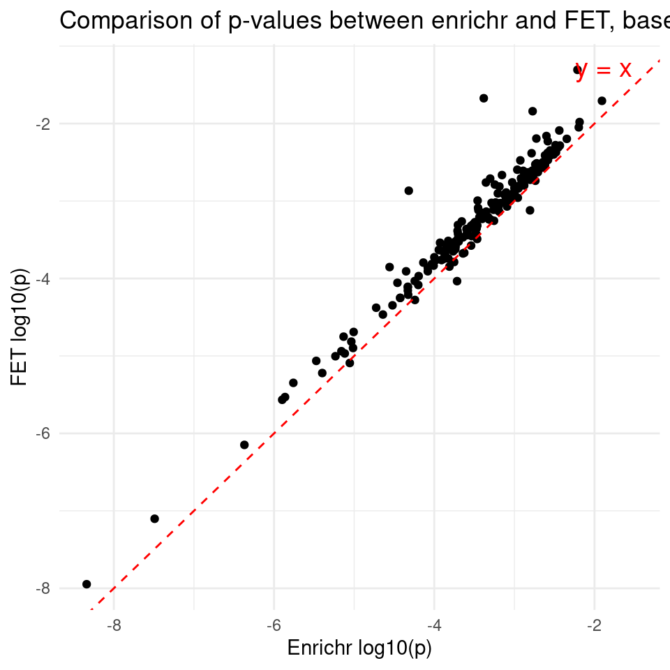
| Version | Author | Date |
|---|---|---|
| ba30ddd | XSun | 2024-10-24 |
Summary for the number of Go terms with p-values < 0.001
 load("/project/xinhe/xsun/multi_group_ctwas/11.multi_group_1008/postprocess/enrichment_summary_for_all_redundant_p.rdata")

summary_show <- summary[grep(pattern = "ctwasgene",summary$method),]

DT::datatable(summary_show,caption = htmltools::tags$caption( style = 'caption-side: topleft; text-align = left; color:black;','Number of enriched GO terms under different settings'),options = list(pageLength = 20) )
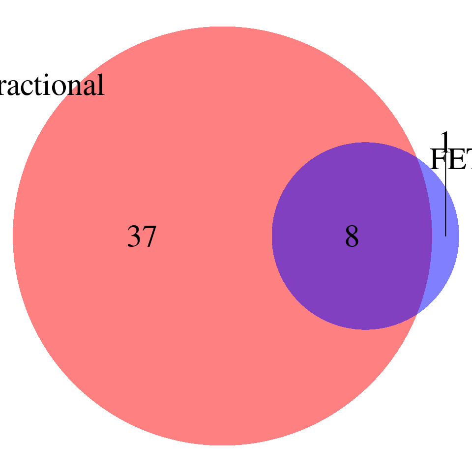
Comparing the GO terms reported by FET and Fractional model (pvalues calibrated) – p-values < 0.001, baseline genes are genes used in ctwas, redundant terms NOT removed
aFib-ebi-a-GCST006414
all_fractional <- c()
all_fet <- c()

trait <- "aFib-ebi-a-GCST006414"

for (db in dbs) {

    file_fet <- paste0("/project/xinhe/xsun/multi_group_ctwas/11.multi_group_1008/postprocess/enrichment_fisher_blctwas_pip08_",trait,"_",db,".rdata")
    load(file_fet)
    all_fet <- rbind(all_fet,summary)

    file_fractional <- paste0("/project/xinhe/xsun/multi_group_ctwas/11.multi_group_1008/postprocess/enrichment_fractional_calibrated_",trait,"_",db,".rdata")
    load(file_fractional)
    summary$trait <- trait
    summary$db <- db
    all_fractional <- rbind(all_fractional,summary)

}

all_fractional$id <- paste0(all_fractional$trait,"-",all_fractional$db,"-",all_fractional$GO)
all_fet$id <- paste0(all_fet$trait,"-",all_fet$db,"-",all_fet$GO)

fractional_pass <- all_fractional[as.numeric(all_fractional$pvalue_calibrated) < pval_threshold, ]
fractional_pass <-  fractional_pass[complete.cases( fractional_pass$fdr_origin),]
fet_pass <- all_fet[as.numeric(all_fet$pvalue) < pval_threshold, ]

venn.plot <- draw.pairwise.venn(
     area1 = nrow(fractional_pass),          # Size of Group A
     area2 = nrow(fet_pass),          # Size of Group B
     cross.area = sum(fractional_pass$id %in%  fet_pass$id),     # Overlap between Group A and Group B
     category = c("Fractional", "FET"),  # Labels for the groups
     fill = c("red", "blue"),             # Colors for the groups
     lty = "blank",                       # Line type for the circles
     cex = 2,                             # Font size for the numbers
     cat.cex = 2                          # Font size for the labels
   )
| Version | Author | Date |
|---|---|---|
| 2446887 | XSun | 2024-10-23 |
all_fractional <- all_fractional[,c("trait","db","GO","pvalue_origin","fdr_origin","pvalue_calibrated","fdr_calibrated","id")]

merged_two <- merge(all_fractional,all_fet, by = "id")
merged_two <- merged_two[,c("trait.x","db.x","GO.x","pvalue_origin","fdr_origin","pvalue_calibrated","fdr_calibrated","pvalue","fdr","Overlap","Genes")]
colnames(merged_two) <- c("trait","db","GO","pvalue_origin_fractional","fdr_origin_fractional","pvalue_calibrated_fractional","fdr_calibrated_fractional","pvalue_fet","fdr_fet","Overlap_fet","Overlapped_Genes_fet")
unique_fractional <- merged_two[as.numeric(merged_two$pvalue_calibrated_fractional) < pval_threshold & as.numeric(merged_two$pvalue_fet) > pval_threshold,]
unique_fractional <- unique_fractional[complete.cases(unique_fractional),]
unique_fractional <- unique_fractional[order(as.numeric(unique_fractional$pvalue_calibrated_fractional)),]
DT::datatable(unique_fractional,caption = htmltools::tags$caption( style = 'caption-side: topleft; text-align = left; color:black;','Unique GO terms for fractional model'),options = list(pageLength = 10) )
unique_fet<- merged_two[as.numeric(merged_two$pvalue_calibrated_fractional) > pval_threshold & as.numeric(merged_two$pvalue_fet) < pval_threshold,]
unique_fet <- unique_fet[complete.cases(unique_fet),]
DT::datatable(unique_fet,caption = htmltools::tags$caption( style = 'caption-side: topleft; text-align = left; color:black;','Unique GO terms for FET'),options = list(pageLength = 10) )p_fractional_calibrated <- as.numeric(unique_fractional$pvalue_calibrated_fractional)
p_fet <- as.numeric(unique_fractional$pvalue_fet)
lgp_fractional_calibrated <- log10(p_fractional_calibrated)
lgp_fet <- log10(p_fet)
df <- data.frame(lgp_fractional_calibrated = lgp_fractional_calibrated, lgp_fet = lgp_fet)
ggplot(df, aes(x = lgp_fractional_calibrated, y = lgp_fet)) +
geom_point() + # Add points
geom_abline(intercept = 0, slope = 1, color = "red", linetype = "dashed") + # y = x line
#geom_smooth(method = "lm", se = FALSE, color = "blue") + # Best-fit line
# annotate("text", x = max(lgp_fractional_calibrated) * 0.8, y = max(lgp_fet) * 0.9,
# label = paste0("Slope: ", round(slope, 3)),
# color = "blue") + # Slope text
annotate("text", x = max(lgp_fractional_calibrated) * 0.8, y = max(lgp_fractional_calibrated) * 0.8,
label = "y = x", color = "red", size = 5, hjust = 1, vjust = -0.5) + # y = x text near the line
ggtitle("Comparison of p-values between \n fractional_calibrated and FET \n for unique fractional GO terms") + # Add title
xlab("fractional_calibrated log10(p)") + # x-axis label
ylab("FET log10(p)") + # y-axis label
theme_minimal()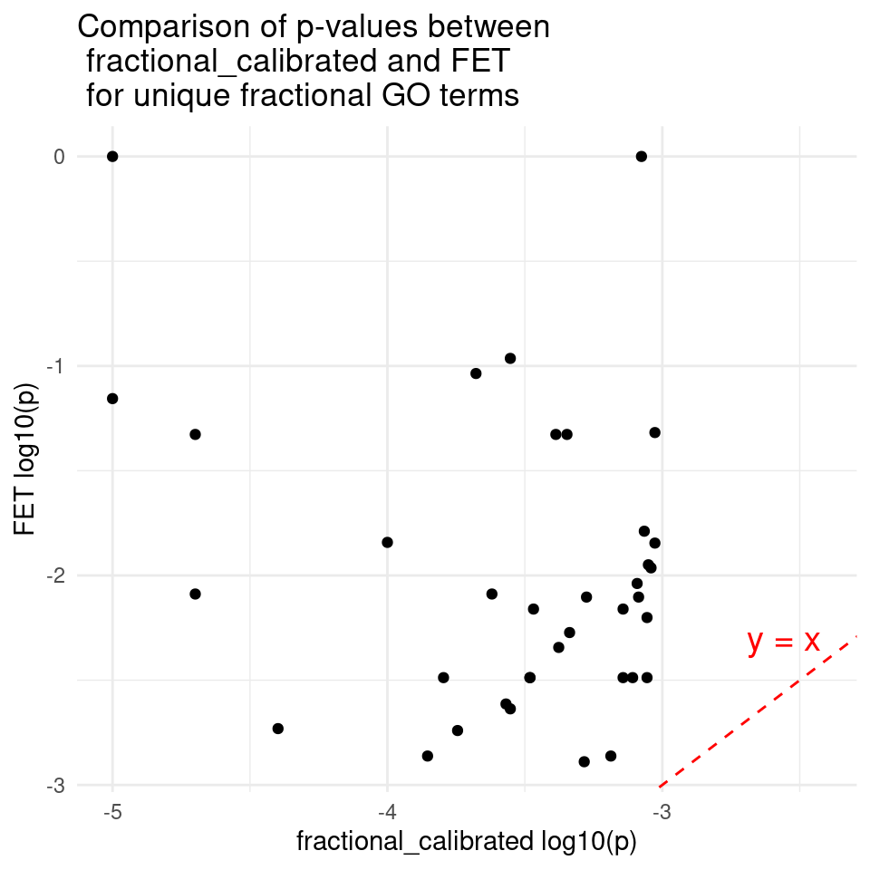
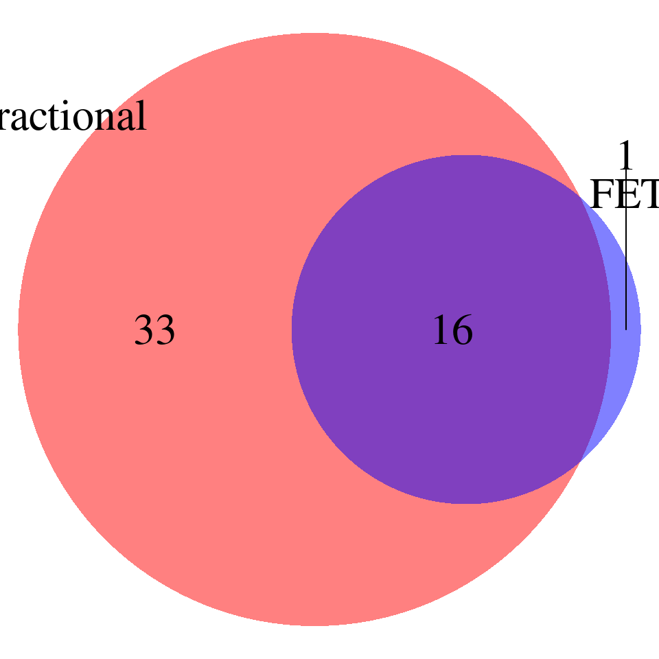
LDL-ukb-d-30780_irnt
all_fractional <- c()
all_fet <- c()

trait <- "LDL-ukb-d-30780_irnt"

for (db in dbs) {

    file_fet <- paste0("/project/xinhe/xsun/multi_group_ctwas/11.multi_group_1008/postprocess/enrichment_fisher_blctwas_pip08_",trait,"_",db,".rdata")
    load(file_fet)
    all_fet <- rbind(all_fet,summary)

    file_fractional <- paste0("/project/xinhe/xsun/multi_group_ctwas/11.multi_group_1008/postprocess/enrichment_fractional_calibrated_",trait,"_",db,".rdata")
    load(file_fractional)
    summary$trait <- trait
    summary$db <- db
    all_fractional <- rbind(all_fractional,summary)

}

all_fractional$id <- paste0(all_fractional$trait,"-",all_fractional$db,"-",all_fractional$GO)
all_fet$id <- paste0(all_fet$trait,"-",all_fet$db,"-",all_fet$GO)

fractional_pass <- all_fractional[as.numeric(all_fractional$pvalue_calibrated) < pval_threshold, ]
fractional_pass <-  fractional_pass[complete.cases( fractional_pass$fdr_origin),]
fet_pass <- all_fet[as.numeric(all_fet$pvalue) < pval_threshold, ]

venn.plot <- draw.pairwise.venn(
     area1 = nrow(fractional_pass),          # Size of Group A
     area2 = nrow(fet_pass),          # Size of Group B
     cross.area = sum(fractional_pass$id %in%  fet_pass$id),     # Overlap between Group A and Group B
     category = c("Fractional", "FET"),  # Labels for the groups
     fill = c("red", "blue"),             # Colors for the groups
     lty = "blank",                       # Line type for the circles
     cex = 2,                             # Font size for the numbers
     cat.cex = 2                          # Font size for the labels
   )
| Version | Author | Date |
|---|---|---|
| 2446887 | XSun | 2024-10-23 |
all_fractional <- all_fractional[,c("trait","db","GO","pvalue_origin","fdr_origin","pvalue_calibrated","fdr_calibrated","id")]

merged_two <- merge(all_fractional,all_fet, by = "id")
merged_two <- merged_two[,c("trait.x","db.x","GO.x","pvalue_origin","fdr_origin","pvalue_calibrated","fdr_calibrated","pvalue","fdr","Overlap","Genes")]
colnames(merged_two) <- c("trait","db","GO","pvalue_origin_fractional","fdr_origin_fractional","pvalue_calibrated_fractional","fdr_calibrated_fractional","pvalue_fet","fdr_fet","Overlap_fet","Overlapped_Genes_fet")
unique_fractional <- merged_two[as.numeric(merged_two$pvalue_calibrated_fractional) < pval_threshold & as.numeric(merged_two$pvalue_fet) > pval_threshold,]
unique_fractional <- unique_fractional[complete.cases(unique_fractional),]
unique_fractional <- unique_fractional[order(as.numeric(unique_fractional$pvalue_calibrated_fractional)),]
DT::datatable(unique_fractional,caption = htmltools::tags$caption( style = 'caption-side: topleft; text-align = left; color:black;','Unique GO terms for fractional model'),options = list(pageLength = 10) )
unique_fet<- merged_two[as.numeric(merged_two$pvalue_calibrated_fractional) > pval_threshold & as.numeric(merged_two$pvalue_fet) < pval_threshold,]
unique_fet <- unique_fet[complete.cases(unique_fet),]
DT::datatable(unique_fet,caption = htmltools::tags$caption( style = 'caption-side: topleft; text-align = left; color:black;','Unique GO terms for FET'),options = list(pageLength = 10) )p_fractional_calibrated <- as.numeric(unique_fractional$pvalue_calibrated_fractional)
p_fet <- as.numeric(unique_fractional$pvalue_fet)
lgp_fractional_calibrated <- log10(p_fractional_calibrated)
lgp_fet <- log10(p_fet)
df <- data.frame(lgp_fractional_calibrated = lgp_fractional_calibrated, lgp_fet = lgp_fet)
ggplot(df, aes(x = lgp_fractional_calibrated, y = lgp_fet)) +
geom_point() + # Add points
geom_abline(intercept = 0, slope = 1, color = "red", linetype = "dashed") + # y = x line
#geom_smooth(method = "lm", se = FALSE, color = "blue") + # Best-fit line
# annotate("text", x = max(lgp_fractional_calibrated) * 0.8, y = max(lgp_fet) * 0.9,
# label = paste0("Slope: ", round(slope, 3)),
# color = "blue") + # Slope text
annotate("text", x = max(lgp_fractional_calibrated) * 0.8, y = max(lgp_fractional_calibrated) * 0.8,
label = "y = x", color = "red", size = 5, hjust = 1, vjust = -0.5) + # y = x text near the line
ggtitle("Comparison of p-values between \n fractional_calibrated and FET \n for unique fractional GO terms") + # Add title
xlab("fractional_calibrated log10(p)") + # x-axis label
ylab("FET log10(p)") + # y-axis label
theme_minimal()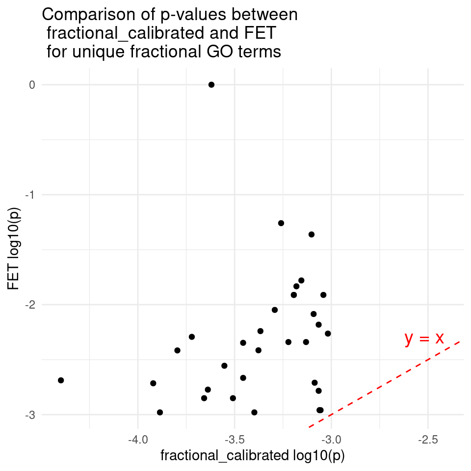
sessionInfo()R version 4.2.0 (2022-04-22)
Platform: x86_64-pc-linux-gnu (64-bit)
Running under: CentOS Linux 7 (Core)
Matrix products: default
BLAS/LAPACK: /software/openblas-0.3.13-el7-x86_64/lib/libopenblas_haswellp-r0.3.13.so
locale:
[1] C
attached base packages:
[1] grid stats graphics grDevices utils datasets methods
[8] base
other attached packages:
[1] ggplot2_3.5.1 VennDiagram_1.7.3 futile.logger_1.4.3
[4] dplyr_1.1.4 tidyr_1.3.0
loaded via a namespace (and not attached):
[1] tidyselect_1.2.0 xfun_0.41 bslib_0.3.1
[4] purrr_1.0.2 colorspace_2.0-3 vctrs_0.6.5
[7] generics_0.1.2 htmltools_0.5.2 yaml_2.3.5
[10] utf8_1.2.2 rlang_1.1.2 jquerylib_0.1.4
[13] later_1.3.0 pillar_1.9.0 glue_1.6.2
[16] withr_2.5.0 lambda.r_1.2.4 lifecycle_1.0.4
[19] stringr_1.5.1 munsell_0.5.0 gtable_0.3.0
[22] workflowr_1.7.0 htmlwidgets_1.5.4 evaluate_0.15
[25] labeling_0.4.2 knitr_1.39 fastmap_1.1.0
[28] crosstalk_1.2.0 httpuv_1.6.5 fansi_1.0.3
[31] highr_0.9 Rcpp_1.0.12 promises_1.2.0.1
[34] scales_1.3.0 DT_0.22 formatR_1.12
[37] jsonlite_1.8.0 farver_2.1.0 fs_1.5.2
[40] digest_0.6.29 stringi_1.7.6 rprojroot_2.0.3
[43] cli_3.6.1 tools_4.2.0 magrittr_2.0.3
[46] sass_0.4.1 tibble_3.2.1 futile.options_1.0.1
[49] whisker_0.4 pkgconfig_2.0.3 rmarkdown_2.25
[52] rstudioapi_0.13 R6_2.5.1 git2r_0.30.1
[55] compiler_4.2.0