Compare LD mismatch filterng on real data
Kaixuan Luo
2024-01-19
Last updated: 2024-01-19
Checks: 7 0
Knit directory: multigroup_ctwas_analysis/
This reproducible R Markdown analysis was created with workflowr (version 1.7.0). The Checks tab describes the reproducibility checks that were applied when the results were created. The Past versions tab lists the development history.
Great! Since the R Markdown file has been committed to the Git repository, you know the exact version of the code that produced these results.
Great job! The global environment was empty. Objects defined in the global environment can affect the analysis in your R Markdown file in unknown ways. For reproduciblity it’s best to always run the code in an empty environment.
The command set.seed(20231112) was run prior to running the code in the R Markdown file. Setting a seed ensures that any results that rely on randomness, e.g. subsampling or permutations, are reproducible.
Great job! Recording the operating system, R version, and package versions is critical for reproducibility.
Nice! There were no cached chunks for this analysis, so you can be confident that you successfully produced the results during this run.
Great job! Using relative paths to the files within your workflowr project makes it easier to run your code on other machines.
Great! You are using Git for version control. Tracking code development and connecting the code version to the results is critical for reproducibility.
The results in this page were generated with repository version 9c640ec. See the Past versions tab to see a history of the changes made to the R Markdown and HTML files.
Note that you need to be careful to ensure that all relevant files for the analysis have been committed to Git prior to generating the results (you can use wflow_publish or wflow_git_commit). workflowr only checks the R Markdown file, but you know if there are other scripts or data files that it depends on. Below is the status of the Git repository when the results were generated:
Ignored files:
    Ignored:    .Rhistory
    Ignored:    .Rproj.user/
Note that any generated files, e.g. HTML, png, CSS, etc., are not included in this status report because it is ok for generated content to have uncommitted changes.
These are the previous versions of the repository in which changes were made to the R Markdown (analysis/compare_LD_mismatch_filtering_real_data.Rmd) and HTML (docs/compare_LD_mismatch_filtering_real_data.html) files. If you’ve configured a remote Git repository (see ?wflow_git_remote), click on the hyperlinks in the table below to view the files as they were in that past version.
| File | Version | Author | Date | Message |
|---|---|---|---|---|
| Rmd | 9c640ec | kevinlkx | 2024-01-19 | added notes about the locus plots |
Load packages and functions
library(ctwas)
library(ggplot2)
library(tidyverse)
# This section requires internet connections
library(biomaRt)
# download all entries for ensembl on all chromosomes
ensembl <- useEnsembl(biomart="ENSEMBL_MART_ENSEMBL", dataset="hsapiens_gene_ensembl")
G_list <- getBM(filters= "chromosome_name", attributes= c("hgnc_symbol","chromosome_name","start_position","end_position","gene_biotype", "ensembl_gene_id", "strand"), values=1:22, mart=ensembl)
table(G_list$chromosome_name)
# subset to protein coding genes and fix empty gene names
G_list <- G_list[G_list$gene_biotype %in% c("protein_coding"),]
G_list$hgnc_symbol[G_list$hgnc_symbol==""] <- "-"
# set TSS based on start/end position and strand
G_list$tss <- G_list[,c("end_position", "start_position")][cbind(1:nrow(G_list),G_list$strand/2+1.5)]
save(G_list, file="/project2/xinhe/kevinluo/cTWAS/data/G_list_allchrs.RData")LDL
trait <- "LDL"
tissue <- "Liver"
gwas_name <- "LDL-ukb-d-30780_irnt"
gwas_n <- 343621
thin <- 0.1
max_snp_region <- 20000

tissue <- R.utils::capitalize(tissue)
ld_R_dir <- "/project2/mstephens/wcrouse/UKB_LDR_0.1/"
Weight
weight_name <- paste0("mashr_", tissue, "_nolnc")
weight <- paste0("/project2/xinhe/shared_data/multigroup_ctwas/weights/predictdb_nolnc/", weight_name, ".db")
cat("weight: \n")
print(weight)

# Preharmonize prediction models and LD reference
strand_ambig_action <- "drop"
outputdir <- paste0("/project2/xinhe/kevinluo/cTWAS/multigroup/cTWAS_filter_ld_mismatch/", trait, "/")
weight <- file.path(outputdir, paste0(weight_name, "_harmonized_weights_", strand_ambig_action, ".db"))
cat("harmonized weight: \n")
print(weight)
# weight:
# [1] "/project2/xinhe/shared_data/multigroup_ctwas/weights/predictdb_nolnc/mashr_Liver_nolnc.db"
# harmonized weight:
# [1] "/project2/xinhe/kevinluo/cTWAS/multigroup/cTWAS_filter_ld_mismatch/LDL//mashr_Liver_nolnc_harmonized_weights_drop.db"Without filtering
outputdir <- paste0("/project2/xinhe/kevinluo/cTWAS/multigroup/cTWAS_filter_ld_mismatch/", trait, "/")
filter_method <- "none"
outname <- paste0(trait, ".", tissue, ".", filter_method, "_filter")

ctwas_none_filtering_parameters <- ctwas_summarize_parameters(outputdir = outputdir,
                                                              outname = outname,
                                                              gwas_n = gwas_n,
                                                              thin = thin)

ctwas_none_filtering_parameters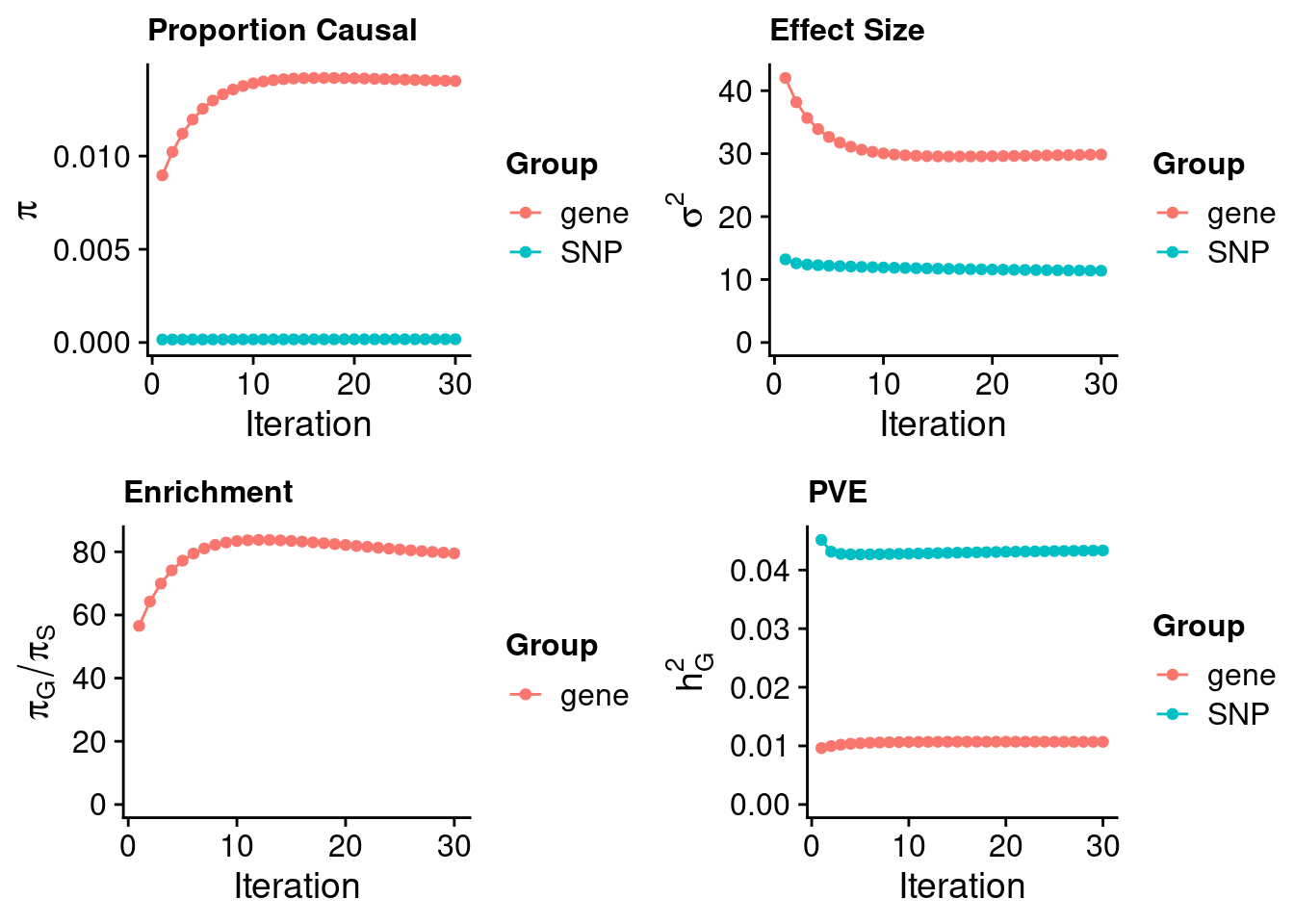
# $group_size
#     SNP    gene
# 7405450    8775
#
# $group_prior
#          SNP         gene
# 0.0001764255 0.0140266909
#
# $group_prior_var
#      SNP     gene
# 11.39814 29.85853
#
# $enrichment
#     gene
# 79.50488
#
# $group_pve
#        SNP       gene
# 0.04333785 0.01069525
#
# $total_pve
# [1] 0.0540331
#
# $attributable_pve
#       SNP      gene
# 0.8020611 0.1979389
#
# $convergence_plot
# load cTWAS results
ctwas_res <- data.table::fread(paste0(outputdir, outname, ".susieIrss.txt"), header=T)
load(file.path(outputdir, paste0(outname, "_z_snp_harmonized_", strand_ambig_action, ".Rd")))
load(file.path(outputdir, paste0(outname, "_z_gene.Rd")))
# load gene information from PredictDB
sqlite <- RSQLite::dbDriver("SQLite")
db = RSQLite::dbConnect(sqlite, weight)
query <- function(...) RSQLite::dbGetQuery(db, ...)
gene_info <- query("select gene, genename, gene_type from extra")
RSQLite::dbDisconnect(db)
# add gene names to cTWAS results
ctwas_res$genename[ctwas_res$type=="gene"] <- gene_info$genename[match(ctwas_res$id[ctwas_res$type=="gene"], gene_info$gene)]
# add z-scores to cTWAS results
ctwas_res$z[ctwas_res$type=="SNP"] <- z_snp$z[match(ctwas_res$id[ctwas_res$type=="SNP"], z_snp$id)]
ctwas_res$z[ctwas_res$type=="gene"] <- z_gene$z[match(ctwas_res$id[ctwas_res$type=="gene"], z_gene$id)]
# display the genes with PIP > 0.8
ctwas_res <- ctwas_res[order(-ctwas_res$susie_pip),]
ctwas_none_filtering_gene_res <- ctwas_res[ctwas_res$type=="gene",]
ctwas_none_filtering_highpip_gene_res <- ctwas_res[ctwas_res$type=="gene" & ctwas_res$susie_pip > 0.8,]
cat(length(unique(ctwas_none_filtering_highpip_gene_res$genename)), "genes with PIP > 0.8. \n")
# update the position for each gene to the TSS.
load(file="/project2/xinhe/kevinluo/cTWAS/data/G_list_allchrs.RData")
# remove the version number from the ensembl IDs
ctwas_res$ensembl <- NA
ctwas_res$ensembl[ctwas_res$type=="gene"] <- sapply(ctwas_res$id[ctwas_res$type=="gene"], function(x){unlist(strsplit(x, "[.]"))[1]})
#update the gene positions to TSS
ctwas_res$pos[ctwas_res$type=="gene"] <- G_list$tss[match(ctwas_res$ensembl[ctwas_res$type=="gene"], G_list$ensembl_gene_id)]
ctwas_none_filtering_res <- ctwas_res# 45 genes with PIP > 0.8.DENTIST filtering
outputdir <- paste0("/project2/xinhe/kevinluo/cTWAS/multigroup/cTWAS_filter_ld_mismatch/", trait, "/")
filter_method <- "DENTIST"
outname <- paste0(trait, ".", tissue, ".", filter_method, "_filter")

ctwas_dentist_parameters <- ctwas_summarize_parameters(outputdir = outputdir,
                                                       outname = outname,
                                                       gwas_n = gwas_n,
                                                       thin = thin)

ctwas_dentist_parameters
# $group_size
#     SNP    gene
# 7405290    8774
#
# $group_prior
#         SNP        gene
# 0.000176426 0.014026648
#
# $group_prior_var
#      SNP     gene
# 11.39815 29.85859
#
# $enrichment
#     gene
# 79.50441
#
# $group_pve
#        SNP       gene
# 0.04333707 0.01069402
#
# $total_pve
# [1] 0.0540311
#
# $attributable_pve
#       SNP      gene
# 0.8020765 0.1979235
#
# $convergence_plot
# load cTWAS results
ctwas_res <- data.table::fread(paste0(outputdir, outname, ".susieIrss.txt"), header=T)
load(file.path(outputdir, paste0(outname, "_z_snp_harmonized_", strand_ambig_action, ".Rd")))
load(file.path(outputdir, paste0(outname, "_z_gene.Rd")))
# load gene information from PredictDB
sqlite <- RSQLite::dbDriver("SQLite")
db = RSQLite::dbConnect(sqlite, weight)
query <- function(...) RSQLite::dbGetQuery(db, ...)
gene_info <- query("select gene, genename, gene_type from extra")
RSQLite::dbDisconnect(db)
# add gene names to cTWAS results
ctwas_res$genename[ctwas_res$type=="gene"] <- gene_info$genename[match(ctwas_res$id[ctwas_res$type=="gene"], gene_info$gene)]
# add z-scores to cTWAS results
ctwas_res$z[ctwas_res$type=="SNP"] <- z_snp$z[match(ctwas_res$id[ctwas_res$type=="SNP"], z_snp$id)]
ctwas_res$z[ctwas_res$type=="gene"] <- z_gene$z[match(ctwas_res$id[ctwas_res$type=="gene"], z_gene$id)]
# display the genes with PIP > 0.8
ctwas_res <- ctwas_res[order(-ctwas_res$susie_pip),]
ctwas_dentist_gene_res <- ctwas_res[ctwas_res$type=="gene",]
ctwas_dentist_highpip_gene_res <- ctwas_res[ctwas_res$type=="gene" & ctwas_res$susie_pip > 0.8,]
cat(length(unique(ctwas_dentist_highpip_gene_res$genename)), "genes with PIP > 0.8. \n")
# update the position for each gene to the TSS.
load(file="/project2/xinhe/kevinluo/cTWAS/data/G_list_allchrs.RData")
# remove the version number from the ensembl IDs
ctwas_res$ensembl <- NA
ctwas_res$ensembl[ctwas_res$type=="gene"] <- sapply(ctwas_res$id[ctwas_res$type=="gene"], function(x){unlist(strsplit(x, "[.]"))[1]})
#update the gene positions to TSS
ctwas_res$pos[ctwas_res$type=="gene"] <- G_list$tss[match(ctwas_res$ensembl[ctwas_res$type=="gene"], G_list$ensembl_gene_id)]
ctwas_dentist_res <- ctwas_res# 45 genes with PIP > 0.8.SuSiE filtering
outputdir <- paste0("/project2/xinhe/kevinluo/cTWAS/multigroup/cTWAS_filter_ld_mismatch/", trait, "/")
filter_method <- "SuSiE"
outname <- paste0(trait, ".", tissue, ".", filter_method, "_filter")

ctwas_susie_parameters <- ctwas_summarize_parameters(outputdir = outputdir,
                                                     outname = outname,
                                                     gwas_n = gwas_n,
                                                     thin = thin)

ctwas_susie_parameters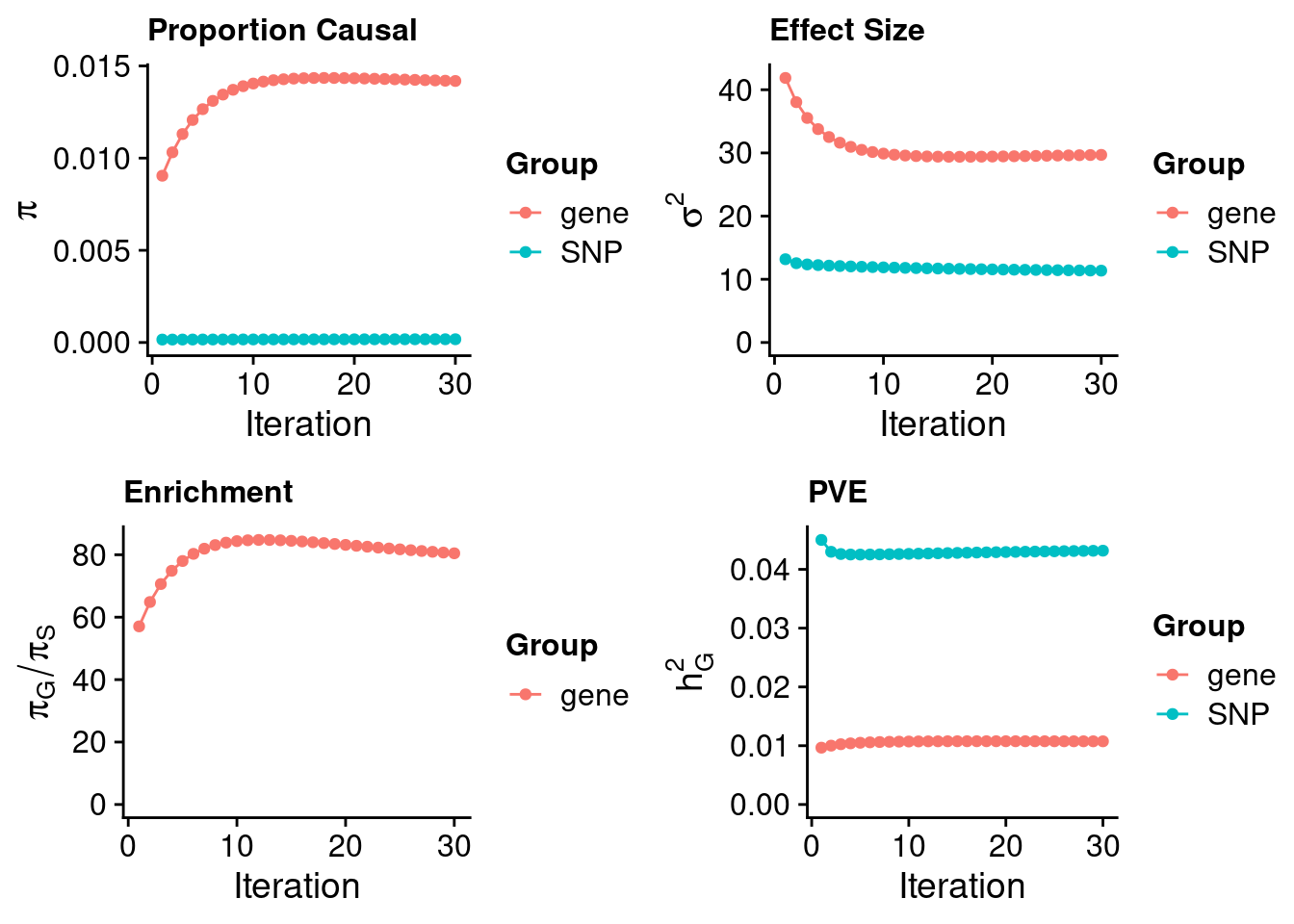
# $group_size
#     SNP    gene
# 7401640    8770
#
# $group_prior
#          SNP         gene
# 0.0001762665 0.0141830628
#
# $group_prior_var
#      SNP     gene
# 11.37163 29.69081
#
# $enrichment
#     gene
# 80.46372
#
# $group_pve
#        SNP       gene
# 0.04317585 0.01074761
#
# $total_pve
# [1] 0.05392346
#
# $attributable_pve
#       SNP      gene
# 0.8006877 0.1993123
#
# $convergence_plot
# load cTWAS results
ctwas_res <- data.table::fread(paste0(outputdir, outname, ".susieIrss.txt"), header=T)
load(file.path(outputdir, paste0(outname, "_z_snp_harmonized_", strand_ambig_action, ".Rd")))
load(file.path(outputdir, paste0(outname, "_z_gene.Rd")))
# load gene information from PredictDB
sqlite <- RSQLite::dbDriver("SQLite")
db = RSQLite::dbConnect(sqlite, weight)
query <- function(...) RSQLite::dbGetQuery(db, ...)
gene_info <- query("select gene, genename, gene_type from extra")
RSQLite::dbDisconnect(db)
# add gene names to cTWAS results
ctwas_res$genename[ctwas_res$type=="gene"] <- gene_info$genename[match(ctwas_res$id[ctwas_res$type=="gene"], gene_info$gene)]
# add z-scores to cTWAS results
ctwas_res$z[ctwas_res$type=="SNP"] <- z_snp$z[match(ctwas_res$id[ctwas_res$type=="SNP"], z_snp$id)]
ctwas_res$z[ctwas_res$type=="gene"] <- z_gene$z[match(ctwas_res$id[ctwas_res$type=="gene"], z_gene$id)]
# display the genes with PIP > 0.8
ctwas_res <- ctwas_res[order(-ctwas_res$susie_pip),]
ctwas_susie_gene_res <- ctwas_res[ctwas_res$type=="gene",]
ctwas_susie_highpip_gene_res <- ctwas_res[ctwas_res$type=="gene" & ctwas_res$susie_pip > 0.8,]
cat(length(unique(ctwas_susie_highpip_gene_res$genename)), "genes with PIP > 0.8. \n")
# update the position for each gene to the TSS.
load(file="/project2/xinhe/kevinluo/cTWAS/data/G_list_allchrs.RData")
# remove the version number from the ensembl IDs
ctwas_res$ensembl <- NA
ctwas_res$ensembl[ctwas_res$type=="gene"] <- sapply(ctwas_res$id[ctwas_res$type=="gene"], function(x){unlist(strsplit(x, "[.]"))[1]})
#update the gene positions to TSS
ctwas_res$pos[ctwas_res$type=="gene"] <- G_list$tss[match(ctwas_res$ensembl[ctwas_res$type=="gene"], G_list$ensembl_gene_id)]
ctwas_susie_res <- ctwas_res# 45 genes with PIP > 0.8.Summary
df <- ctwas_none_filtering_gene_res[, c("id", "type", "genename")]
df$pip_none_filtering <- ctwas_none_filtering_gene_res$susie_pip
df$pip_dentist_filtering <- ctwas_dentist_gene_res$susie_pip[match(df$id, ctwas_dentist_gene_res$id)]
df$pip_susie_filtering <- ctwas_susie_gene_res$susie_pip[match(df$id, ctwas_susie_gene_res$id)]

ggplot(data = df, aes(x = pip_none_filtering, y = pip_dentist_filtering)) +
  geom_point() +
  geom_abline(intercept = 0, slope = 1, col = "red") +
  labs(x = "gene PIP without filtering", y = "gene PIP with DENTIST filtering") +
  theme_bw()
# Warning: Removed 1 rows containing missing values (`geom_point()`).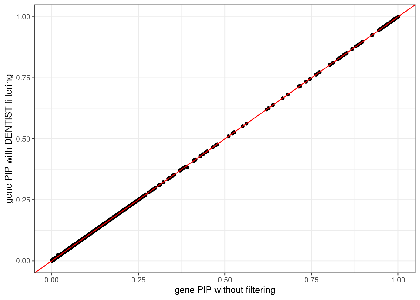
ggplot(data = df, aes(x = pip_none_filtering, y = pip_susie_filtering)) +
  geom_point() +
  geom_abline(intercept = 0, slope = 1, col = "red") +
  labs(x = "gene PIP without filtering", y = "gene PIP with SuSiE filtering") +
  theme_bw()
# Warning: Removed 5 rows containing missing values (`geom_point()`).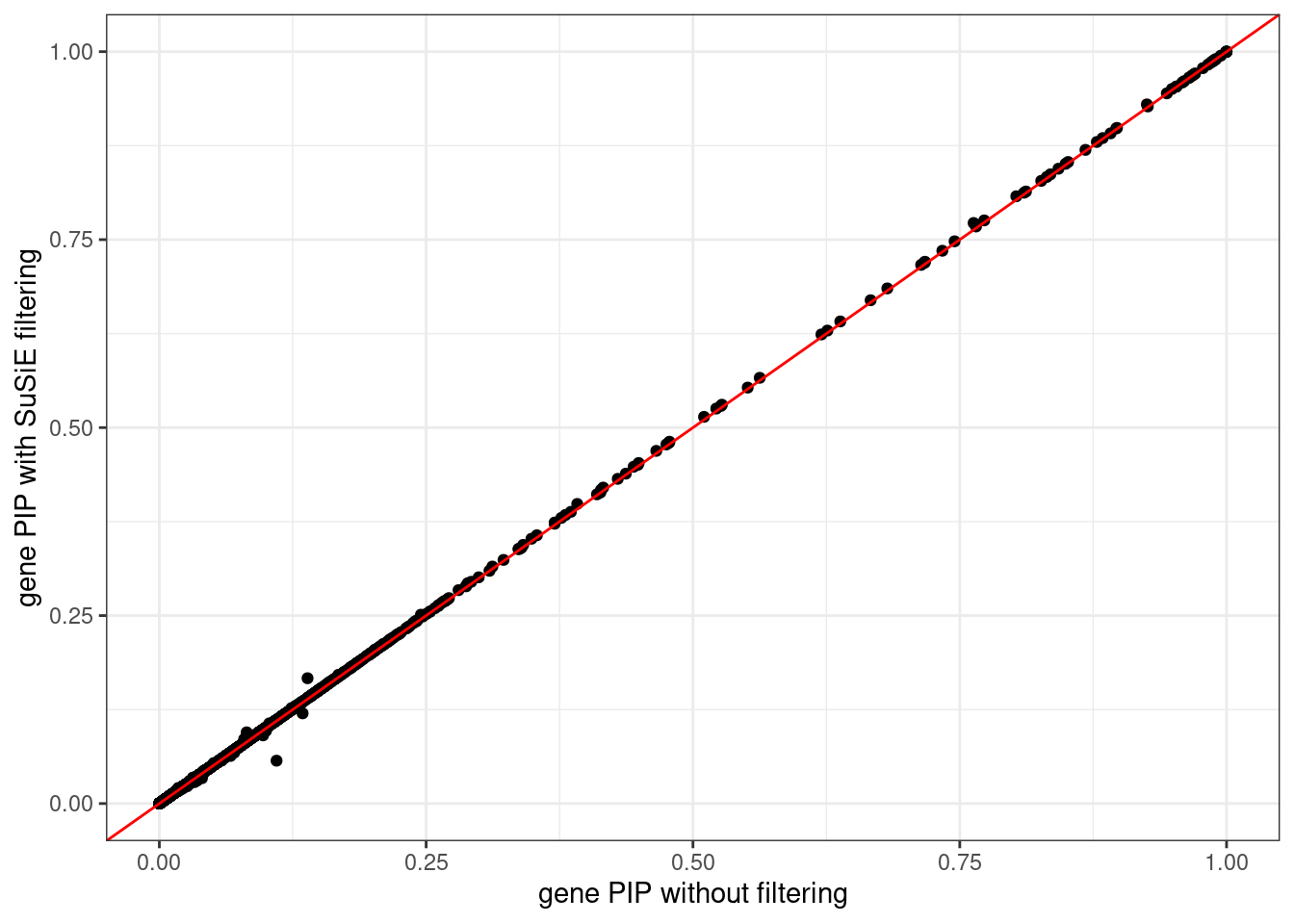
ggplot(data = df, aes(x = pip_dentist_filtering, y = pip_susie_filtering)) +
  geom_point() +
  geom_abline(intercept = 0, slope = 1, col = "red") +
  labs(x = "gene PIP with DENTIST filtering", y = "gene PIP with SuSiE filtering") +
  theme_bw()
# Warning: Removed 6 rows containing missing values (`geom_point()`).
aFib
trait <- "aFib"
tissue <- "Heart_Atrial_Appendage"
gwas_name <- "aFib-ebi-a-GCST006414"
gwas_n <- 1030836
thin <- 0.1
max_snp_region <- 20000

tissue <- R.utils::capitalize(tissue)
ld_R_dir <- "/project2/mstephens/wcrouse/UKB_LDR_0.1/"
Weight
weight_name <- paste0("mashr_", tissue, "_nolnc")
weight <- paste0("/project2/xinhe/shared_data/multigroup_ctwas/weights/predictdb_nolnc/", weight_name, ".db")
cat("weight: \n")
print(weight)

# Preharmonize prediction models and LD reference
strand_ambig_action <- "drop"
outputdir <- paste0("/project2/xinhe/kevinluo/cTWAS/multigroup/cTWAS_filter_ld_mismatch/", trait, "/")
weight <- file.path(outputdir, paste0(weight_name, "_harmonized_weights_", strand_ambig_action, ".db"))
cat("harmonized weight: \n")
print(weight)
# weight:
# [1] "/project2/xinhe/shared_data/multigroup_ctwas/weights/predictdb_nolnc/mashr_Heart_Atrial_Appendage_nolnc.db"
# harmonized weight:
# [1] "/project2/xinhe/kevinluo/cTWAS/multigroup/cTWAS_filter_ld_mismatch/aFib//mashr_Heart_Atrial_Appendage_nolnc_harmonized_weights_drop.db"Without filtering
outputdir <- paste0("/project2/xinhe/kevinluo/cTWAS/multigroup/cTWAS_filter_ld_mismatch/", trait, "/")
filter_method <- "none"
outname <- paste0(trait, ".", tissue, ".", filter_method, "_filter")

ctwas_none_filtering_parameters <- ctwas_summarize_parameters(outputdir = outputdir,
                                                              outname = outname,
                                                              gwas_n = gwas_n,
                                                              thin = thin)

ctwas_none_filtering_parameters
# $group_size
#     SNP    gene
# 7055050    9894
#
# $group_prior
#          SNP         gene
# 0.0001818829 0.0238113548
#
# $group_prior_var
#       SNP      gene
#  8.613486 10.430038
#
# $enrichment
#     gene
# 130.9159
#
# $group_pve
#         SNP        gene
# 0.010722136 0.002383704
#
# $total_pve
# [1] 0.01310584
#
# $attributable_pve
#      SNP     gene
# 0.818119 0.181881
#
# $convergence_plot
# load cTWAS results
ctwas_res <- data.table::fread(paste0(outputdir, outname, ".susieIrss.txt"), header=T)
load(file.path(outputdir, paste0(outname, "_z_snp_harmonized_", strand_ambig_action, ".Rd")))
load(file.path(outputdir, paste0(outname, "_z_gene.Rd")))
# load gene information from PredictDB
sqlite <- RSQLite::dbDriver("SQLite")
db = RSQLite::dbConnect(sqlite, weight)
query <- function(...) RSQLite::dbGetQuery(db, ...)
gene_info <- query("select gene, genename, gene_type from extra")
RSQLite::dbDisconnect(db)
# add gene names to cTWAS results
ctwas_res$genename[ctwas_res$type=="gene"] <- gene_info$genename[match(ctwas_res$id[ctwas_res$type=="gene"], gene_info$gene)]
# add z-scores to cTWAS results
ctwas_res$z[ctwas_res$type=="SNP"] <- z_snp$z[match(ctwas_res$id[ctwas_res$type=="SNP"], z_snp$id)]
ctwas_res$z[ctwas_res$type=="gene"] <- z_gene$z[match(ctwas_res$id[ctwas_res$type=="gene"], z_gene$id)]
# display the genes with PIP > 0.8
ctwas_res <- ctwas_res[order(-ctwas_res$susie_pip),]
ctwas_none_filtering_gene_res <- ctwas_res[ctwas_res$type=="gene",]
ctwas_none_filtering_highpip_gene_res <- ctwas_res[ctwas_res$type=="gene" & ctwas_res$susie_pip > 0.8,]
cat(length(unique(ctwas_none_filtering_highpip_gene_res$genename)), "genes with PIP > 0.8. \n")
# update the position for each gene to the TSS.
load(file="/project2/xinhe/kevinluo/cTWAS/data/G_list_allchrs.RData")
# remove the version number from the ensembl IDs
ctwas_res$ensembl <- NA
ctwas_res$ensembl[ctwas_res$type=="gene"] <- sapply(ctwas_res$id[ctwas_res$type=="gene"], function(x){unlist(strsplit(x, "[.]"))[1]})
#update the gene positions to TSS
ctwas_res$pos[ctwas_res$type=="gene"] <- G_list$tss[match(ctwas_res$ensembl[ctwas_res$type=="gene"], G_list$ensembl_gene_id)]
ctwas_none_filtering_res <- ctwas_res# 42 genes with PIP > 0.8.DENTIST filtering
outputdir <- paste0("/project2/xinhe/kevinluo/cTWAS/multigroup/cTWAS_filter_ld_mismatch/", trait, "/")
filter_method <- "DENTIST"
outname <- paste0(trait, ".", tissue, ".", filter_method, "_filter")

ctwas_dentist_parameters <- ctwas_summarize_parameters(outputdir = outputdir,
                                                       outname = outname,
                                                       gwas_n = gwas_n,
                                                       thin = thin)

ctwas_dentist_parameters
# $group_size
#     SNP    gene
# 6790540    9711
#
# $group_prior
#          SNP         gene
# 0.0001998022 0.0218272229
#
# $group_prior_var
#       SNP      gene
#  8.001629 12.391268
#
# $enrichment
#     gene
# 109.2442
#
# $group_pve
#         SNP        gene
# 0.010531577 0.002547937
#
# $total_pve
# [1] 0.01307951
#
# $attributable_pve
#       SNP      gene
# 0.8051964 0.1948036
#
# $convergence_plot
# load cTWAS results
ctwas_res <- data.table::fread(paste0(outputdir, outname, ".susieIrss.txt"), header=T)
load(file.path(outputdir, paste0(outname, "_z_snp_harmonized_", strand_ambig_action, ".Rd")))
load(file.path(outputdir, paste0(outname, "_z_gene.Rd")))
# load gene information from PredictDB
sqlite <- RSQLite::dbDriver("SQLite")
db = RSQLite::dbConnect(sqlite, weight)
query <- function(...) RSQLite::dbGetQuery(db, ...)
gene_info <- query("select gene, genename, gene_type from extra")
RSQLite::dbDisconnect(db)
# add gene names to cTWAS results
ctwas_res$genename[ctwas_res$type=="gene"] <- gene_info$genename[match(ctwas_res$id[ctwas_res$type=="gene"], gene_info$gene)]
# add z-scores to cTWAS results
ctwas_res$z[ctwas_res$type=="SNP"] <- z_snp$z[match(ctwas_res$id[ctwas_res$type=="SNP"], z_snp$id)]
ctwas_res$z[ctwas_res$type=="gene"] <- z_gene$z[match(ctwas_res$id[ctwas_res$type=="gene"], z_gene$id)]
# display the genes with PIP > 0.8
ctwas_res <- ctwas_res[order(-ctwas_res$susie_pip),]
ctwas_dentist_gene_res <- ctwas_res[ctwas_res$type=="gene",]
ctwas_dentist_highpip_gene_res <- ctwas_res[ctwas_res$type=="gene" & ctwas_res$susie_pip > 0.8,]
cat(length(unique(ctwas_dentist_highpip_gene_res$genename)), "genes with PIP > 0.8. \n")
# update the position for each gene to the TSS.
load(file="/project2/xinhe/kevinluo/cTWAS/data/G_list_allchrs.RData")
# remove the version number from the ensembl IDs
ctwas_res$ensembl <- NA
ctwas_res$ensembl[ctwas_res$type=="gene"] <- sapply(ctwas_res$id[ctwas_res$type=="gene"], function(x){unlist(strsplit(x, "[.]"))[1]})
#update the gene positions to TSS
ctwas_res$pos[ctwas_res$type=="gene"] <- G_list$tss[match(ctwas_res$ensembl[ctwas_res$type=="gene"], G_list$ensembl_gene_id)]
ctwas_dentist_res <- ctwas_res# 44 genes with PIP > 0.8.SuSiE filtering
outputdir <- paste0("/project2/xinhe/kevinluo/cTWAS/multigroup/cTWAS_filter_ld_mismatch/", trait, "/")
filter_method <- "SuSiE"
outname <- paste0(trait, ".", tissue, ".", filter_method, "_filter")

ctwas_susie_parameters <- ctwas_summarize_parameters(outputdir = outputdir,
                                                     outname = outname,
                                                     gwas_n = gwas_n,
                                                     thin = thin)

ctwas_susie_parameters
# $group_size
#     SNP    gene
# 7024770    9863
#
# $group_prior
#          SNP         gene
# 0.0001840401 0.0237465422
#
# $group_prior_var
#       SNP      gene
#  8.562658 10.404694
#
# $enrichment
#     gene
# 129.0291
#
# $group_pve
#         SNP        gene
# 0.010738996 0.002364009
#
# $total_pve
# [1] 0.01310301
#
# $attributable_pve
#       SNP      gene
# 0.8195827 0.1804173
#
# $convergence_plot
# load cTWAS results
ctwas_res <- data.table::fread(paste0(outputdir, outname, ".susieIrss.txt"), header=T)
load(file.path(outputdir, paste0(outname, "_z_snp_harmonized_", strand_ambig_action, ".Rd")))
load(file.path(outputdir, paste0(outname, "_z_gene.Rd")))
# load gene information from PredictDB
sqlite <- RSQLite::dbDriver("SQLite")
db = RSQLite::dbConnect(sqlite, weight)
query <- function(...) RSQLite::dbGetQuery(db, ...)
gene_info <- query("select gene, genename, gene_type from extra")
RSQLite::dbDisconnect(db)
# add gene names to cTWAS results
ctwas_res$genename[ctwas_res$type=="gene"] <- gene_info$genename[match(ctwas_res$id[ctwas_res$type=="gene"], gene_info$gene)]
# add z-scores to cTWAS results
ctwas_res$z[ctwas_res$type=="SNP"] <- z_snp$z[match(ctwas_res$id[ctwas_res$type=="SNP"], z_snp$id)]
ctwas_res$z[ctwas_res$type=="gene"] <- z_gene$z[match(ctwas_res$id[ctwas_res$type=="gene"], z_gene$id)]
# display the genes with PIP > 0.8
ctwas_res <- ctwas_res[order(-ctwas_res$susie_pip),]
ctwas_susie_gene_res <- ctwas_res[ctwas_res$type=="gene",]
ctwas_susie_highpip_gene_res <- ctwas_res[ctwas_res$type=="gene" & ctwas_res$susie_pip > 0.8,]
cat(length(unique(ctwas_susie_highpip_gene_res$genename)), "genes with PIP > 0.8. \n")
# update the position for each gene to the TSS.
load(file="/project2/xinhe/kevinluo/cTWAS/data/G_list_allchrs.RData")
# remove the version number from the ensembl IDs
ctwas_res$ensembl <- NA
ctwas_res$ensembl[ctwas_res$type=="gene"] <- sapply(ctwas_res$id[ctwas_res$type=="gene"], function(x){unlist(strsplit(x, "[.]"))[1]})
#update the gene positions to TSS
ctwas_res$pos[ctwas_res$type=="gene"] <- G_list$tss[match(ctwas_res$ensembl[ctwas_res$type=="gene"], G_list$ensembl_gene_id)]
ctwas_susie_res <- ctwas_res# 43 genes with PIP > 0.8.Summary
df <- ctwas_none_filtering_gene_res[, c("id", "type", "genename")]
df$pip_none_filtering <- ctwas_none_filtering_gene_res$susie_pip
df$pip_dentist_filtering <- ctwas_dentist_gene_res$susie_pip[match(df$id, ctwas_dentist_gene_res$id)]
df$pip_susie_filtering <- ctwas_susie_gene_res$susie_pip[match(df$id, ctwas_susie_gene_res$id)]

ggplot(data = df, aes(x = pip_none_filtering, y = pip_dentist_filtering)) +
  geom_point() +
  geom_abline(intercept = 0, slope = 1, col = "red") +
  labs(x = "gene PIP without filtering", y = "gene PIP with DENTIST filtering") +
  theme_bw()
# Warning: Removed 183 rows containing missing values (`geom_point()`).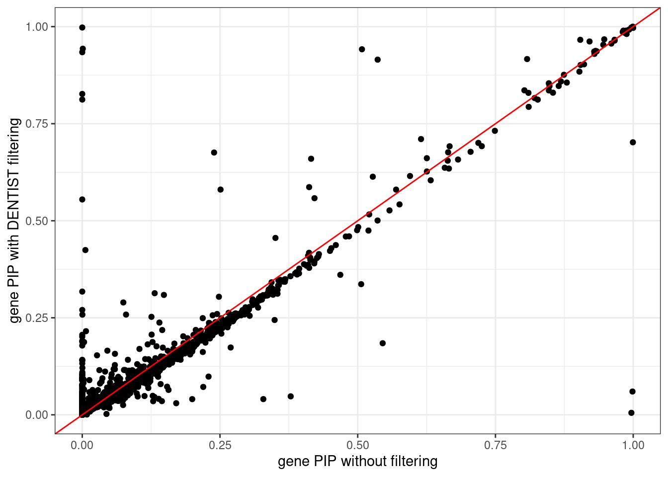
ggplot(data = df, aes(x = pip_none_filtering, y = pip_susie_filtering)) +
  geom_point() +
  geom_abline(intercept = 0, slope = 1, col = "red") +
  labs(x = "gene PIP without filtering", y = "gene PIP with SuSiE filtering") +
  theme_bw()
# Warning: Removed 31 rows containing missing values (`geom_point()`).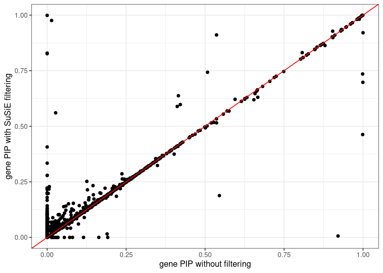
ggplot(data = df, aes(x = pip_dentist_filtering, y = pip_susie_filtering)) +
  geom_point() +
  geom_abline(intercept = 0, slope = 1, col = "red") +
  labs(x = "gene PIP with DENTIST filtering", y = "gene PIP with SuSiE filtering") +
  theme_bw()
# Warning: Removed 187 rows containing missing values (`geom_point()`).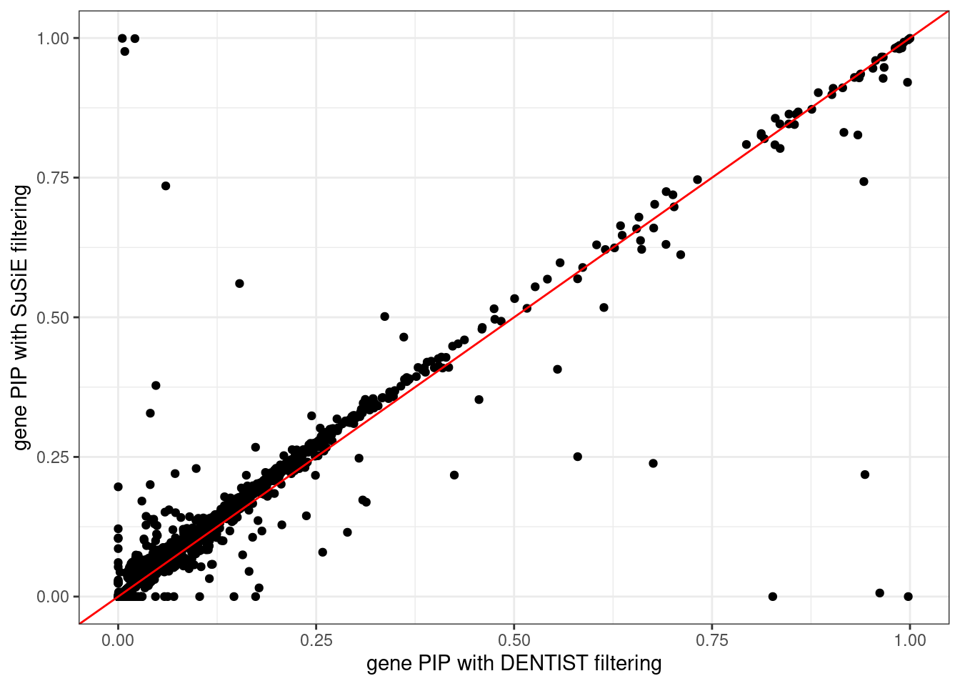
Example locus plots
df <- ctwas_none_filtering_gene_res[, c("id", "type", "genename")]
df$pip_none_filtering <- ctwas_none_filtering_gene_res$susie_pip
df$pip_dentist_filtering <- ctwas_dentist_gene_res$susie_pip[match(df$id, ctwas_dentist_gene_res$id)]
df$pip_susie_filtering <- ctwas_susie_gene_res$susie_pip[match(df$id, ctwas_susie_gene_res$id)]

# df[order(df$pip_none_filtering- df$pip_dentist_filtering)[1:5],]
#
# df[order(df$pip_none_filtering- df$pip_susie_filtering)[1:5],]
#
# df[order(df$pip_dentist_filtering - df$pip_none_filtering)[1:5],]
#
# df[order(df$pip_susie_filtering - df$pip_none_filtering)[1:5],]
CAV2 locus
CAV2 gene PIP increased significantly after DENTIST filtering.
print(df[df$genename == "CAV2",])# id type genename pip_none_filtering pip_dentist_filtering
# 1: ENSG00000105971.14 gene CAV2 1.233718e-06 0.9978039
# pip_susie_filtering
# 1: 7.774559e-12without filtering
# genome-wide bonferroni threshold used for TWAS
twas_sig_thresh <- 0.05/sum(ctwas_none_filtering_res$type=="gene")

# show cTWAS result for CAV2 and store region_tag
print(ctwas_none_filtering_res[which(ctwas_none_filtering_res$genename=="CAV2"),])
region_tag <- "7_70"

# make locus plot
ctwas_locus_plot(ctwas_res = ctwas_none_filtering_res,
                 region_tag = region_tag,
                 xlim = c(115,117),
                 twas_sig_thresh = twas_sig_thresh,
                 alt_names = "genename", #the column that specify gene names
                 legend_panel = "TWAS", #the panel to plot legend
                 legend_side="left", #the position of the panel
                 outputdir = outputdir,
                 outname = outname)
# Warning in asMethod(object): sparse->dense coercion: allocating vector of size
# 2.7 GiB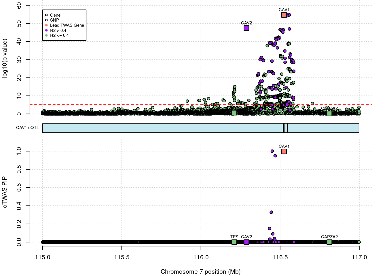
#    chrom                 id       pos type region_tag1 region_tag2 cs_index
# 1:     7 ENSG00000105971.14 116287380 gene           7          70        0
#       susie_pip      mu2 genename         z         ensembl
# 1: 1.233718e-06 3044.044     CAV2 -14.58049 ENSG00000105971
DENTIST result
# genome-wide bonferroni threshold used for TWAS
twas_sig_thresh <- 0.05/sum(ctwas_dentist_res$type=="gene")

# show cTWAS result for CAV2 and store region_tag
print(ctwas_dentist_res[which(ctwas_dentist_res$genename=="CAV2"),])
region_tag <- "7_70"

# make locus plot
ctwas_locus_plot(ctwas_res = ctwas_dentist_res,
                 region_tag = region_tag,
                 xlim = c(115,117),
                 twas_sig_thresh = twas_sig_thresh,
                 alt_names = "genename", #the column that specify gene names
                 legend_panel = "TWAS", #the panel to plot legend
                 legend_side="left", #the position of the panel
                 outputdir = outputdir,
                 outname = outname)
# Warning in asMethod(object): sparse->dense coercion: allocating vector of size
# 2.7 GiB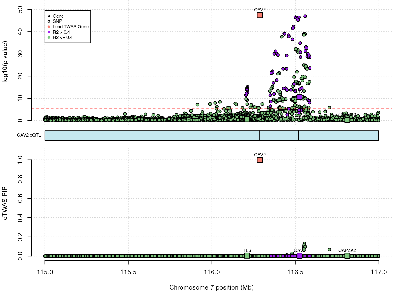
#    chrom                 id       pos type region_tag1 region_tag2 cs_index
# 1:     7 ENSG00000105971.14 116287380 gene           7          70        1
#    susie_pip    mu2 genename         z         ensembl
# 1: 0.9978039 123.94     CAV2 -14.58049 ENSG00000105971
cTWAS results for CAV1 and CAV2
cat("without filtering: \n")
ctwas_none_filtering_res %>%
  filter(region_tag1 == 7, region_tag2 == 70, genename %in% c("CAV1", "CAV2")) %>%
  arrange(genename)

cat("DENTIST filtering: \n")
ctwas_dentist_res %>%
  filter(region_tag1 == 7, region_tag2 == 70, genename %in% c("CAV1", "CAV2")) %>%
  arrange(genename)
# without filtering:
# chrom id pos type region_tag1 region_tag2 cs_index
# 1: 7 ENSG00000105974.11 116524994 gene 7 70 1
# 2: 7 ENSG00000105971.14 116287380 gene 7 70 0
# susie_pip mu2 genename z ensembl
# 1: 9.967226e-01 2334.597 CAV1 -15.68396 ENSG00000105974
# 2: 1.233718e-06 3044.044 CAV2 -14.58049 ENSG00000105971
# DENTIST filtering:
# chrom id pos type region_tag1 region_tag2 cs_index
# 1: 7 ENSG00000105974.11 116524994 gene 7 70 0
# 2: 7 ENSG00000105971.14 116287380 gene 7 70 1
# susie_pip mu2 genename z ensembl
# 1: 0.005170658 28.56626 CAV1 -6.682749 ENSG00000105974
# 2: 0.997803932 123.93999 CAV2 -14.580488 ENSG00000105971Top cTWAS SNPs or genes.
rs75148240 has PIP of 1 before filtering, but was not in the cTWAS results after DENTIST filtering.
cat("without filtering: \n")
ctwas_none_filtering_res %>%
  filter(region_tag1 == 7, region_tag2 == 70) %>%
  arrange(desc(susie_pip)) %>% head()

cat("DENTIST filtering: \n")
ctwas_dentist_res %>%
  filter(region_tag1 == 7, region_tag2 == 70) %>%
  arrange(desc(susie_pip)) %>% head()

ctwas_dentist_res %>% filter(id %in% "rs75148240")
# without filtering:
# chrom id pos type region_tag1 region_tag2 cs_index
# 1: 7 rs75148240 116450390 SNP 7 70 3
# 2: 7 ENSG00000105974.11 116524994 gene 7 70 1
# 3: 7 rs768108 116468604 SNP 7 70 2
# 4: 7 rs12706089 116444313 SNP 7 70 2
# 5: 7 rs10464649 116433513 SNP 7 70 2
# 6: 7 rs4727831 116453929 SNP 7 70 2
# susie_pip mu2 genename z ensembl
# 1: 1.0000000 4181.515 <NA> -4.446429 <NA>
# 2: 0.9967226 2334.597 CAV1 -15.683957 ENSG00000105974
# 3: 0.9493380 4296.678 <NA> -13.208955 <NA>
# 4: 0.3284571 4257.423 <NA> -13.253731 <NA>
# 5: 0.1493546 4250.944 <NA> -13.238806 <NA>
# 6: 0.0903445 4293.808 <NA> -13.089552 <NA>
# DENTIST filtering:
# chrom id pos type region_tag1 region_tag2 cs_index
# 1: 7 ENSG00000105971.14 116287380 gene 7 70 1
# 2: 7 ENSG00000164604.12 113087778 gene 7 70 0
# 3: 7 rs729949 116554851 SNP 7 70 2
# 4: 7 rs7789117 116554330 SNP 7 70 2
# 5: 7 rs3757732 116553651 SNP 7 70 2
# 6: 7 rs3807992 116557191 SNP 7 70 2
# susie_pip mu2 genename z ensembl
# 1: 0.9978039 123.93999 CAV2 -14.580488 ENSG00000105971
# 2: 0.8266767 22.00660 GPR85 -4.320214 ENSG00000164604
# 3: 0.1327644 86.87929 <NA> 13.207792 <NA>
# 4: 0.1323944 86.87133 <NA> 13.207792 <NA>
# 5: 0.1205627 86.52070 <NA> 13.194805 <NA>
# 6: 0.1023433 85.89123 <NA> 13.168831 <NA>
# Empty data.table (0 rows and 12 cols): chrom,id,pos,type,region_tag1,region_tag2...AGAP5 locus
AGAP5 gene PIP increased significantly after SuSiE filtering.
print(df[df$genename == "AGAP5",])# id type genename pip_none_filtering pip_dentist_filtering
# 1: ENSG00000172650.13 gene AGAP5 0.01400113 0.008348378
# pip_susie_filtering
# 1: 0.9758852without filtering
# genome-wide bonferroni threshold used for TWAS
twas_sig_thresh <- 0.05/sum(ctwas_none_filtering_res$type=="gene")

# show cTWAS result for CAV2 and store region_tag
print(ctwas_none_filtering_res[which(ctwas_none_filtering_res$genename=="AGAP5"),])
region_tag <- "10_49"

# make locus plot
ctwas_locus_plot(ctwas_res = ctwas_none_filtering_res,
                 region_tag = region_tag,
                 xlim = c(73,74.5),
                 twas_sig_thresh = twas_sig_thresh,
                 alt_names = "genename", #the column that specify gene names
                 legend_panel = "TWAS", #the panel to plot legend
                 legend_side="left", #the position of the panel
                 outputdir = outputdir,
                 outname = outname)
# Warning in asMethod(object): sparse->dense coercion: allocating vector of size
# 2.3 GiB
#    chrom                 id      pos type region_tag1 region_tag2 cs_index
# 1:    10 ENSG00000172650.13 73698109 gene          10          49        0
#     susie_pip      mu2 genename         z         ensembl
# 1: 0.01400113 161.1709    AGAP5 -11.51406 ENSG00000172650
SuSiE result
# genome-wide bonferroni threshold used for TWAS
twas_sig_thresh <- 0.05/sum(ctwas_susie_res$type=="gene")

# show cTWAS result for KDM3B and store region_tag
print(ctwas_susie_res[which(ctwas_susie_res$genename=="AGAP5"),])
region_tag <- "10_49"

# make locus plot
ctwas_locus_plot(ctwas_res = ctwas_susie_res,
                 region_tag = region_tag,
                 xlim = c(73,74.5),
                 twas_sig_thresh = twas_sig_thresh,
                 alt_names = "genename", #the column that specify gene names
                 legend_panel = "TWAS", #the panel to plot legend
                 legend_side="left", #the position of the panel
                 outputdir = outputdir,
                 outname = outname)
# Warning in asMethod(object): sparse->dense coercion: allocating vector of size
# 2.3 GiB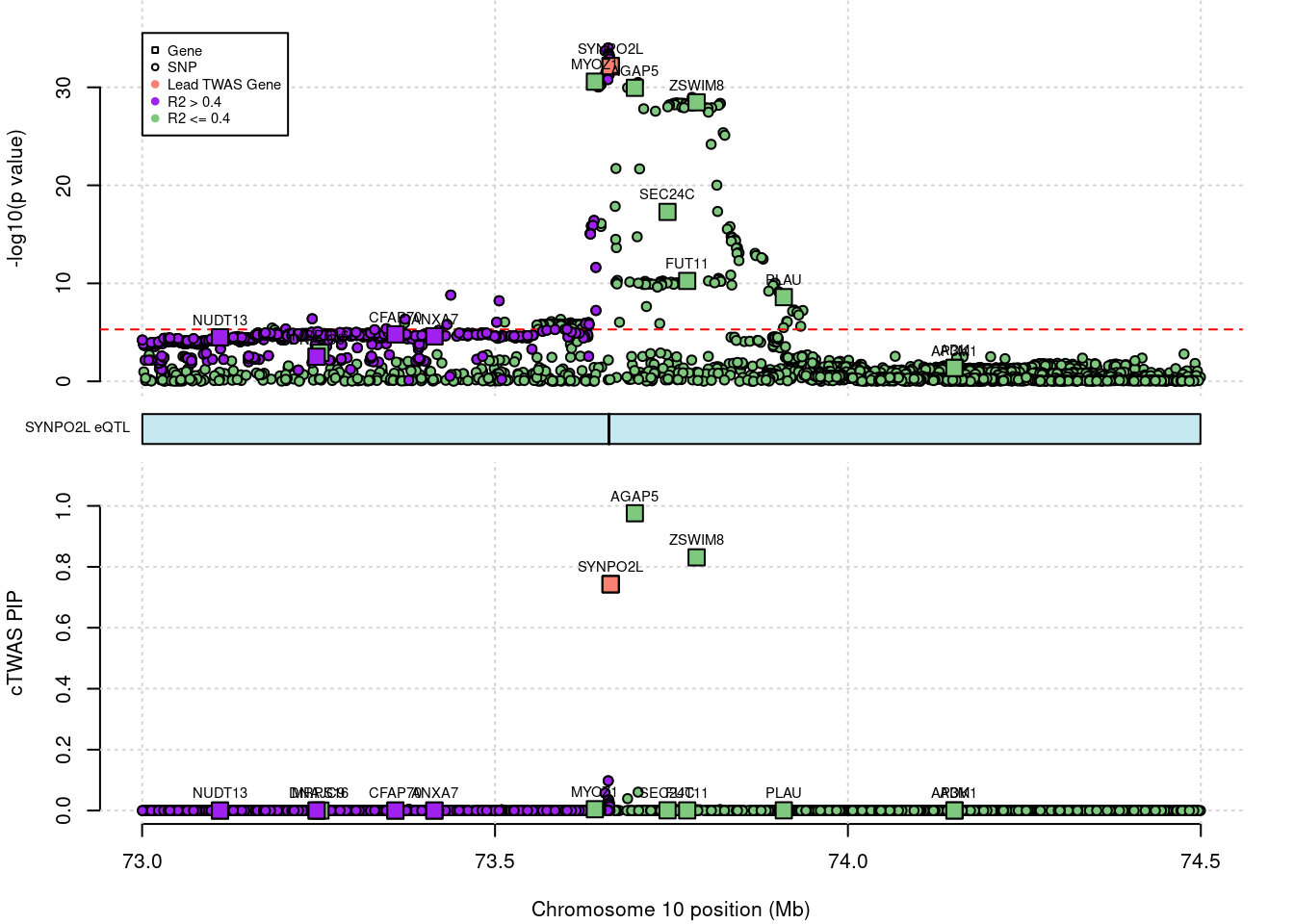
#    chrom                 id      pos type region_tag1 region_tag2 cs_index
# 1:    10 ENSG00000172650.13 73698109 gene          10          49        5
#    susie_pip      mu2 genename         z         ensembl
# 1: 0.9758852 48.99834    AGAP5 -11.51406 ENSG00000172650
Top cTWAS SNPs or genes.
rs113478919 has PIP of 0.9 before filtering, but was not in the cTWAS results after SuSiE filtering.
cat("without filtering: \n")
ctwas_none_filtering_res %>%
  filter(region_tag1 == 10, region_tag2 == 49) %>%
  arrange(desc(susie_pip)) %>% head()

cat("SuSiE filtering: \n")
ctwas_susie_res %>%
  filter(region_tag1 == 10, region_tag2 == 49) %>%
  arrange(desc(susie_pip)) %>% head()

ctwas_susie_res %>% filter(id %in% "rs113478919")
# without filtering:
# chrom id pos type region_tag1 region_tag2 cs_index
# 1: 10 rs113478919 73638668 SNP 10 49 5
# 2: 10 ENSG00000214655.10 73785606 gene 10 49 2
# 3: 10 ENSG00000166317.11 73663803 gene 10 49 1
# 4: 10 rs7915134 73660422 SNP 10 49 1
# 5: 10 rs60632610 73655919 SNP 10 49 1
# 6: 10 rs76192127 73702752 SNP 10 49 2
# susie_pip mu2 genename z ensembl
# 1: 0.92386553 147.4895 <NA> 3.474308 <NA>
# 2: 0.80745697 110.0274 ZSWIM8 11.216495 ENSG00000214655
# 3: 0.50769247 270.2822 SYNPO2L 11.945652 ENSG00000166317
# 4: 0.27247441 274.4906 <NA> 12.294737 <NA>
# 5: 0.10650027 272.7413 <NA> 12.239583 <NA>
# 6: 0.09612647 117.2658 <NA> 11.622449 <NA>
# SuSiE filtering:
# chrom id pos type region_tag1 region_tag2 cs_index
# 1: 10 ENSG00000172650.13 73698109 gene 10 49 5
# 2: 10 ENSG00000214655.10 73785606 gene 10 49 2
# 3: 10 ENSG00000166317.11 73663803 gene 10 49 1
# 4: 10 rs7915134 73660422 SNP 10 49 1
# 5: 10 rs76192127 73702752 SNP 10 49 2
# 6: 10 rs60632610 73655919 SNP 10 49 1
# susie_pip mu2 genename z ensembl
# 1: 0.97588519 48.99834 AGAP5 -11.51406 ENSG00000172650
# 2: 0.83095873 87.63650 ZSWIM8 11.21649 ENSG00000214655
# 3: 0.74295217 101.02872 SYNPO2L 11.94565 ENSG00000166317
# 4: 0.09768095 108.89375 <NA> 12.29474 <NA>
# 5: 0.06043253 94.77616 <NA> 11.62245 <NA>
# 6: 0.05736800 107.69696 <NA> 12.23958 <NA>
# Empty data.table (0 rows and 12 cols): chrom,id,pos,type,region_tag1,region_tag2...C9orf3 locus
C9orf3 gene PIP decreased significantly after DENTIST filtering.
print(df[df$genename == "C9orf3",])# id type genename pip_none_filtering pip_dentist_filtering
# 1: ENSG00000148120.16 gene C9orf3 0.9207887 0.9618413
# pip_susie_filtering
# 1: 0.00640381without filtering
# genome-wide bonferroni threshold used for TWAS
twas_sig_thresh <- 0.05/sum(ctwas_none_filtering_res$type=="gene")

# show cTWAS result for CAV2 and store region_tag
print(ctwas_none_filtering_res[which(ctwas_none_filtering_res$genename=="C9orf3"),])
region_tag <- "9_48"

# make locus plot
ctwas_locus_plot(ctwas_res = ctwas_none_filtering_res,
                 region_tag = region_tag,
                 twas_sig_thresh = twas_sig_thresh,
                 alt_names = "genename", #the column that specify gene names
                 legend_panel = "TWAS", #the panel to plot legend
                 legend_side="left", #the position of the panel
                 outputdir = outputdir,
                 outname = outname)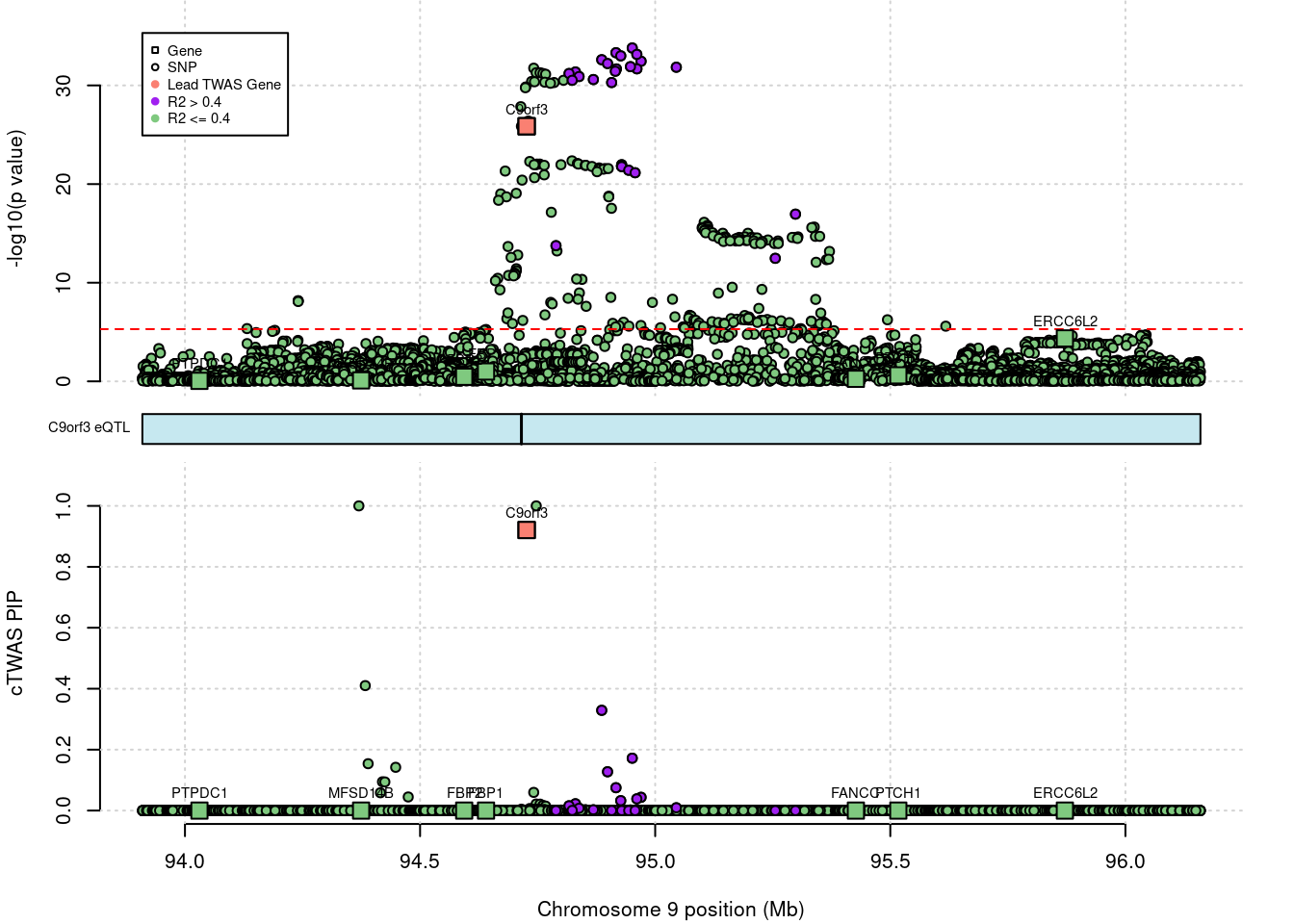
#    chrom                 id      pos type region_tag1 region_tag2 cs_index
# 1:     9 ENSG00000148120.16 94726604 gene           9          48        3
#    susie_pip      mu2 genename         z         ensembl
# 1: 0.9207887 214.7931   C9orf3 -10.67164 ENSG00000148120
SuSiE result
# genome-wide bonferroni threshold used for TWAS
twas_sig_thresh <- 0.05/sum(ctwas_susie_res$type=="gene")

# show cTWAS result for KDM3B and store region_tag
print(ctwas_susie_res[which(ctwas_susie_res$genename=="C9orf3"),])
region_tag <- "9_48"

# make locus plot
ctwas_locus_plot(ctwas_res = ctwas_susie_res,
                 region_tag = region_tag,
                 twas_sig_thresh = twas_sig_thresh,
                 alt_names = "genename", #the column that specify gene names
                 legend_panel = "TWAS", #the panel to plot legend
                 legend_side="left", #the position of the panel
                 outputdir = outputdir,
                 outname = outname)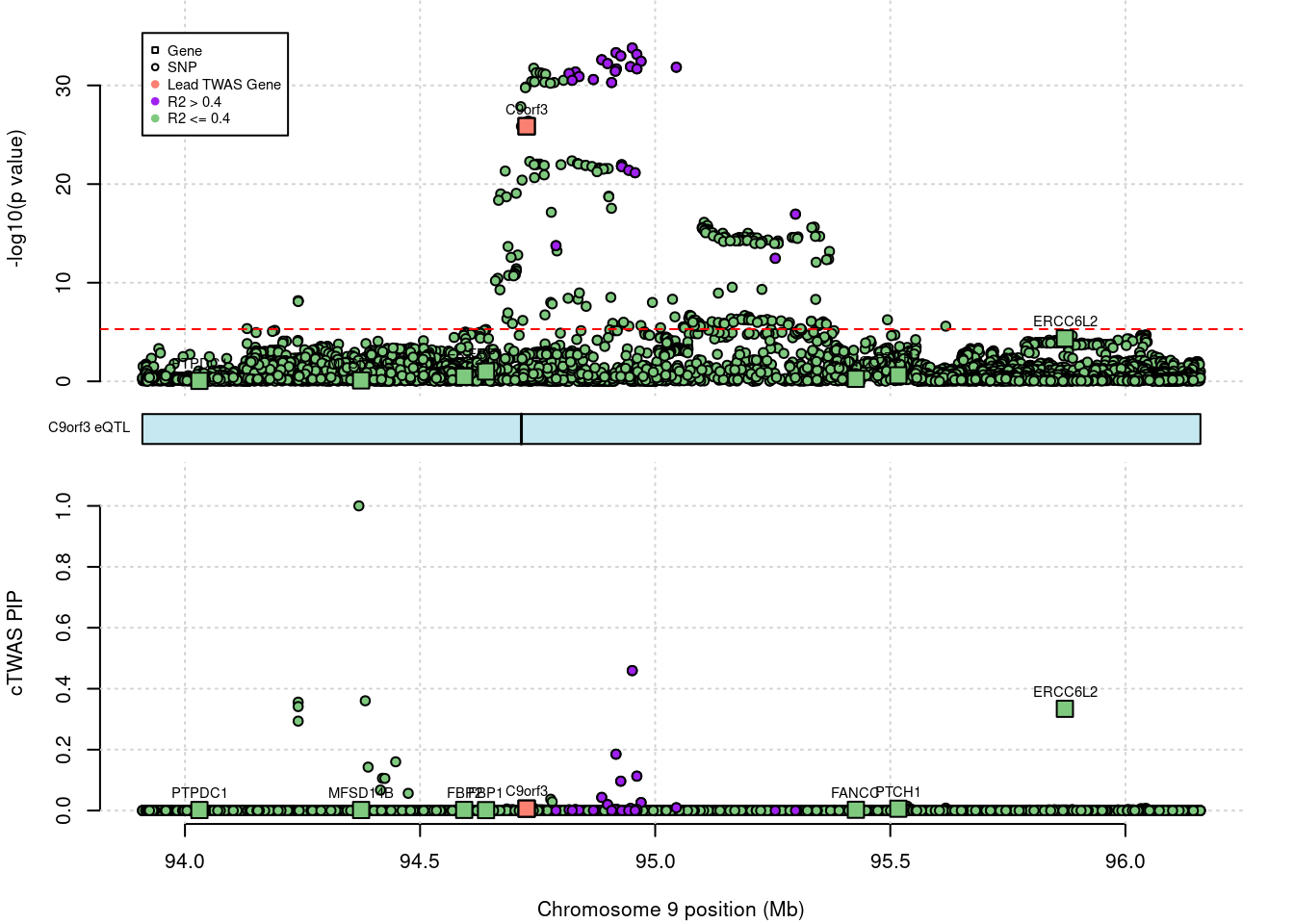
#    chrom                 id      pos type region_tag1 region_tag2 cs_index
# 1:     9 ENSG00000148120.16 94726604 gene           9          48        0
#     susie_pip      mu2 genename         z         ensembl
# 1: 0.00640381 126.1549   C9orf3 -10.67164 ENSG00000148120
Top cTWAS SNPs or genes
cat("without filtering: \n")
ctwas_none_filtering_res %>%
  filter(region_tag1 == 9, region_tag2 == 48) %>%
  arrange(desc(susie_pip)) %>% head()

cat("SuSiE filtering: \n")
ctwas_susie_res %>%
  filter(region_tag1 == 9, region_tag2 == 48) %>%
  arrange(desc(susie_pip)) %>% head()
# without filtering:
# chrom id pos type region_tag1 region_tag2 cs_index
# 1: 9 rs36080252 94369850 SNP 9 48 4
# 2: 9 rs114727539 94747043 SNP 9 48 2
# 3: 9 ENSG00000148120.16 94726604 gene 9 48 3
# 4: 9 rs1831154 94383451 SNP 9 48 5
# 5: 9 rs4385527 94886305 SNP 9 48 1
# 6: 9 rs10821415 94951177 SNP 9 48 1
# susie_pip mu2 genename z ensembl
# 1: 1.0000000 680.5619 <NA> -2.101796 <NA>
# 2: 1.0000000 192.3929 <NA> 3.347150 <NA>
# 3: 0.9207887 214.7931 C9orf3 -10.671642 ENSG00000148120
# 4: 0.4101324 681.3069 <NA> 2.908397 <NA>
# 5: 0.3290236 270.9010 <NA> -12.029851 <NA>
# 6: 0.1718880 264.6791 <NA> -12.253731 <NA>
# SuSiE filtering:
# chrom id pos type region_tag1 region_tag2 cs_index
# 1: 9 rs36080252 94369850 SNP 9 48 3
# 2: 9 rs10821415 94951177 SNP 9 48 1
# 3: 9 rs1831154 94383451 SNP 9 48 4
# 4: 9 rs186999669 94240788 SNP 9 48 5
# 5: 9 rs181926698 94240787 SNP 9 48 5
# 6: 9 ENSG00000182150.15 95871264 gene 9 48 0
# susie_pip mu2 genename z ensembl
# 1: 1.0000000 685.15823 <NA> -2.101796 <NA>
# 2: 0.4594277 159.36628 <NA> -12.253731 <NA>
# 3: 0.3603389 681.31543 <NA> 2.908397 <NA>
# 4: 0.3558851 140.57160 <NA> -5.798387 <NA>
# 5: 0.3412528 140.46264 <NA> -5.790323 <NA>
# 6: 0.3340307 29.21808 ERCC6L2 4.084471 ENSG00000182150
sessionInfo()# R version 4.2.0 (2022-04-22)
# Platform: x86_64-pc-linux-gnu (64-bit)
# Running under: CentOS Linux 7 (Core)
#
# Matrix products: default
# BLAS/LAPACK: /software/openblas-0.3.13-el7-x86_64/lib/libopenblas_haswellp-r0.3.13.so
#
# locale:
# [1] LC_CTYPE=en_US.UTF-8 LC_NUMERIC=C
# [3] LC_TIME=en_US.UTF-8 LC_COLLATE=en_US.UTF-8
# [5] LC_MONETARY=en_US.UTF-8 LC_MESSAGES=en_US.UTF-8
# [7] LC_PAPER=en_US.UTF-8 LC_NAME=C
# [9] LC_ADDRESS=C LC_TELEPHONE=C
# [11] LC_MEASUREMENT=en_US.UTF-8 LC_IDENTIFICATION=C
#
# attached base packages:
# [1] stats graphics grDevices utils datasets methods base
#
# other attached packages:
# [1] cowplot_1.1.1 forcats_1.0.0 stringr_1.5.0 dplyr_1.1.0
# [5] purrr_1.0.1 readr_2.1.4 tidyr_1.3.0 tibble_3.1.8
# [9] tidyverse_1.3.2 ggplot2_3.4.1 ctwas_0.1.35 workflowr_1.7.0
#
# loaded via a namespace (and not attached):
# [1] fs_1.6.1 bit64_4.0.5 lubridate_1.9.2
# [4] httr_1.4.4 rprojroot_2.0.3 tools_4.2.0
# [7] backports_1.4.1 bslib_0.4.2 utf8_1.2.3
# [10] R6_2.5.1 irlba_2.3.5 DBI_1.1.3
# [13] colorspace_2.1-0 withr_2.5.0 tidyselect_1.2.0
# [16] processx_3.8.0 bit_4.0.5 compiler_4.2.0
# [19] git2r_0.30.1 cli_3.6.0 rvest_1.0.3
# [22] logging_0.10-108 xml2_1.3.3 labeling_0.4.2
# [25] sass_0.4.5 scales_1.2.1 callr_3.7.3
# [28] mixsqp_0.3-43 digest_0.6.31 rmarkdown_2.20
# [31] R.utils_2.12.2 pkgconfig_2.0.3 htmltools_0.5.4
# [34] highr_0.10 dbplyr_2.3.0 fastmap_1.1.0
# [37] rlang_1.1.3 readxl_1.4.2 RSQLite_2.2.20
# [40] rstudioapi_0.14 farver_2.1.1 jquerylib_0.1.4
# [43] generics_0.1.3 jsonlite_1.8.4 R.oo_1.25.0
# [46] googlesheets4_1.0.1 magrittr_2.0.3 Matrix_1.5-3
# [49] Rcpp_1.0.10 munsell_0.5.0 fansi_1.0.4
# [52] lifecycle_1.0.3 R.methodsS3_1.8.2 stringi_1.7.12
# [55] whisker_0.4 yaml_2.3.7 blob_1.2.3
# [58] grid_4.2.0 promises_1.2.0.1 crayon_1.5.2
# [61] lattice_0.20-45 haven_2.5.1 hms_1.1.2
# [64] knitr_1.42 ps_1.7.2 pillar_1.8.1
# [67] codetools_0.2-18 reprex_2.0.2 glue_1.6.2
# [70] evaluate_0.20 getPass_0.2-2 data.table_1.14.6
# [73] modelr_0.1.10 vctrs_0.5.2 tzdb_0.3.0
# [76] httpuv_1.6.5 foreach_1.5.2 cellranger_1.1.0
# [79] gtable_0.3.1 pgenlibr_0.3.3 assertthat_0.2.1
# [82] cachem_1.0.6 xfun_0.37 broom_1.0.3
# [85] later_1.3.0 googledrive_2.0.0 gargle_1.3.0
# [88] iterators_1.0.14 memoise_2.0.1 timechange_0.2.0
# [91] ellipsis_0.3.2