Seven Correlated Tissues Simulation
shengqian
2023-12-30
Last updated: 2024-01-15
Checks: 6 1
Knit directory: multigroup_ctwas_analysis/
This reproducible R Markdown analysis was created with workflowr (version 1.7.0). The Checks tab describes the reproducibility checks that were applied when the results were created. The Past versions tab lists the development history.
The R Markdown file has unstaged changes. To know which version of the R Markdown file created these results, you’ll want to first commit it to the Git repo. If you’re still working on the analysis, you can ignore this warning. When you’re finished, you can run wflow_publish to commit the R Markdown file and build the HTML.
Great job! The global environment was empty. Objects defined in the global environment can affect the analysis in your R Markdown file in unknown ways. For reproduciblity it’s best to always run the code in an empty environment.
The command set.seed(20231112) was run prior to running the code in the R Markdown file. Setting a seed ensures that any results that rely on randomness, e.g. subsampling or permutations, are reproducible.
Great job! Recording the operating system, R version, and package versions is critical for reproducibility.
Nice! There were no cached chunks for this analysis, so you can be confident that you successfully produced the results during this run.
Great job! Using relative paths to the files within your workflowr project makes it easier to run your code on other machines.
Great! You are using Git for version control. Tracking code development and connecting the code version to the results is critical for reproducibility.
The results in this page were generated with repository version 3158ac3. See the Past versions tab to see a history of the changes made to the R Markdown and HTML files.
Note that you need to be careful to ensure that all relevant files for the analysis have been committed to Git prior to generating the results (you can use wflow_publish or wflow_git_commit). workflowr only checks the R Markdown file, but you know if there are other scripts or data files that it depends on. Below is the status of the Git repository when the results were generated:
Untracked files:
    Untracked:  analysis/simulation_E_S_one_tissue.Rmd
    Untracked:  analysis/simulation_seven_brain_tissues_correlated.Rmd

Unstaged changes:
    Modified:   analysis/simulation_seven_tissues_correlated.Rmd
Note that any generated files, e.g. HTML, png, CSS, etc., are not included in this status report because it is ok for generated content to have uncommitted changes.
These are the previous versions of the repository in which changes were made to the R Markdown (analysis/simulation_seven_tissues_correlated.Rmd) and HTML (docs/simulation_seven_tissues_correlated.html) files. If you’ve configured a remote Git repository (see ?wflow_git_remote), click on the hyperlinks in the table below to view the files as they were in that past version.
| File | Version | Author | Date | Message |
|---|---|---|---|---|
| Rmd | 4d024a0 | sq-96 | 2024-01-03 | update |
| html | 4d024a0 | sq-96 | 2024-01-03 | update |
| Rmd | 690e29e | sq-96 | 2024-01-03 | update |
| html | 690e29e | sq-96 | 2024-01-03 | update |
| Rmd | 2f6c0dd | sq-96 | 2023-12-30 | update |
| html | 2f6c0dd | sq-96 | 2023-12-30 | update |
| Rmd | 0a32579 | sq-96 | 2023-12-30 | update |
| html | 0a32579 | sq-96 | 2023-12-30 | update |
A simulation of seven correlated tissues is conducted to evaluate cTWAS performance (parameter estimation, PIP calibration …). Seven tissues used in this simulation are Artery Aorta, Spleen, Skin (not sun exposed suprapubic), Lung, Adipose Subcutaneous, Pancreas, Heart Artial Appendage. Pairwise correlation of gene expression are with 0.6-0.8. The first three tissues are set to be causal and the other four tissues are non-causal.
It current has two settings: * 3% PVE, 0.9% \(\pi\) for causal tissues, 0.5% PVE, 0.15% \(\pi\) for non-causal tissues and 30% PVE, 2.5e-4 \(\pi\) for SNP. * 3% PVE, 0.9% \(\pi\) for causal tissues, 0% PVE, 0% \(\pi\) for non-causal tissues and 30% PVE, 2.5e-4 \(\pi\) for SNP.
We observed that cTWAS always tend to overestimate PVE of non-causal tissues because parameters won’t be shrunk exactly to 0. Therefore, we assign non-zero (but very low) PVE to non-causal tissues in the first setting to check if it helps simulation results.
Attaching package: 'ggpubr'The following object is masked from 'package:cowplot':
get_legend
Attaching package: 'plyr'The following object is masked from 'package:ggpubr':
mutateSimulation 1: 3% PVE for Causal Tissues and 0.5% PVE for Non-causal Tissues.
Shared Prior Variance Parameters
For the cTWAS analysis, tissues shared an effect size parameter.
Results using Combined PIP Threshold
  simutag n_causal_combined n_detected_comb_pip n_detected_comb_pip_in_causal
1     1-1               312                  78                            70
2     1-2               345                  88                            77
3     1-3               323                  60                            58
4     1-4               320                  59                            56
5     1-5               302                  55                            51
[1] 0.9176471TWAS results
  simutag n_detected_twas n_detected_twas_in_causal n_detected_comb_twas
1     1-1             647                        81                  235
2     1-2             871                        95                  321
3     1-3             547                        74                  195
4     1-4             583                        64                  227
5     1-5             569                        75                  217
  n_detected_comb_twas_in_causal
1                             84
2                             98
3                             77
4                             64
5                             76
[1] 0.3338912Estimated Prior Inclusion Probability
y1 <- results_df$prior_mashr_Artery_Aorta
y2 <- results_df$prior_mashr_Spleen
y3 <- results_df$prior_mashr_Skin_Not_Sun_Exposed_Suprapubic
y4 <- results_df$prior_mashr_Lung
y5 <- results_df$prior_mashr_Adipose_Subcutaneous
y6 <- results_df$prior_mashr_Pancreas
y7 <- results_df$prior_mashr_Heart_Atrial_Appendage


truth <- rbind(c(1,0.009),c(2,0.009),c(3,0.009),c(4,0.0015),c(5,0.0015),c(6,0.0015),c(7,0.0015))
est <- rbind(cbind(1,y1),cbind(2,y2),cbind(3,y3),cbind(4,y4),cbind(5,y5),cbind(6,y6),cbind(7,y7))
plot_par_7(truth,est,xlabels = c("Artery","Spleen","Skin","Lung","Adipose","Pancreas","Heart"),ylim=c(0,0.025),ylab="Prior inclusion")
Estimated PVE
y1 <- results_df$pve_mashr_Artery_Aorta
y2 <- results_df$pve_mashr_Spleen
y3 <- results_df$pve_mashr_Skin_Not_Sun_Exposed_Suprapubic
y4 <- results_df$pve_mashr_Lung
y5 <- results_df$pve_mashr_Adipose_Subcutaneous
y6 <- results_df$pve_mashr_Pancreas
y7 <- results_df$pve_mashr_Heart_Atrial_Appendage


truth <- rbind(c(1,0.03),c(2,0.03),c(3,0.03),c(4,0.005),c(5,0.005),c(6,0.005),c(7,0.005))
est <- rbind(cbind(1,y1),cbind(2,y2),cbind(3,y3),cbind(4,y4),cbind(5,y5),cbind(6,y6),cbind(7,y7))
plot_par_7(truth,est,xlabels = c("Artery","Spleen","Skin","Lung","Adipose","Pancreas","Heart"),ylim=c(0,0.06),ylab="PVE")
PIP Calibration Plot
f1 <- plot_PIP(configtag, runtag, paste(1, 1:5, sep = "-"), main = "")Warning: Using `size` aesthetic for lines was deprecated in ggplot2 3.4.0.
ℹ Please use `linewidth` instead.
This warning is displayed once every 8 hours.
Call `lifecycle::last_lifecycle_warnings()` to see where this warning was
generated.Warning: The `size` argument of `element_line()` is deprecated as of ggplot2 3.4.0.
ℹ Please use the `linewidth` argument instead.
This warning is displayed once every 8 hours.
Call `lifecycle::last_lifecycle_warnings()` to see where this warning was
generated.f1
Separate effect size parameters
For the cTWAS analysis, each tissue had its own prior inclusion parameter and effect size parameter.
Results using Combined PIP Threshold
  simutag n_causal_combined n_detected_comb_pip n_detected_comb_pip_in_causal
1     1-1               312                  76                            68
2     1-2               345                  88                            76
3     1-3               323                  62                            59
4     1-4               320                  56                            53
5     1-5               302                  54                            50
[1] 0.9107143TWAS results
  simutag n_detected_twas n_detected_twas_in_causal n_detected_comb_twas
1     1-1             647                        81                  235
2     1-2             871                        95                  321
3     1-3             547                        74                  195
4     1-4             583                        64                  227
5     1-5             569                        75                  217
  n_detected_comb_twas_in_causal
1                             84
2                             98
3                             77
4                             64
5                             76
[1] 0.3338912Estimated Prior Inclusion Probability
y1 <- results_df$prior_mashr_Artery_Aorta
y2 <- results_df$prior_mashr_Spleen
y3 <- results_df$prior_mashr_Skin_Not_Sun_Exposed_Suprapubic
y4 <- results_df$prior_mashr_Lung
y5 <- results_df$prior_mashr_Adipose_Subcutaneous
y6 <- results_df$prior_mashr_Pancreas
y7 <- results_df$prior_mashr_Heart_Atrial_Appendage


truth <- rbind(c(1,0.009),c(2,0.009),c(3,0.009),c(4,0.0015),c(5,0.0015),c(6,0.0015),c(7,0.0015))
est <- rbind(cbind(1,y1),cbind(2,y2),cbind(3,y3),cbind(4,y4),cbind(5,y5),cbind(6,y6),cbind(7,y7))
plot_par_7(truth,est,xlabels = c("Artery","Spleen","Skin","Lung","Adipose","Pancreas","Heart"),ylim=c(0,0.025),ylab="Prior inclusion")
Estimated PVE
y1 <- results_df$pve_mashr_Artery_Aorta
y2 <- results_df$pve_mashr_Spleen
y3 <- results_df$pve_mashr_Skin_Not_Sun_Exposed_Suprapubic
y4 <- results_df$pve_mashr_Lung
y5 <- results_df$pve_mashr_Adipose_Subcutaneous
y6 <- results_df$pve_mashr_Pancreas
y7 <- results_df$pve_mashr_Heart_Atrial_Appendage


truth <- rbind(c(1,0.03),c(2,0.03),c(3,0.03),c(4,0.005),c(5,0.005),c(6,0.005),c(7,0.005))
est <- rbind(cbind(1,y1),cbind(2,y2),cbind(3,y3),cbind(4,y4),cbind(5,y5),cbind(6,y6),cbind(7,y7))
plot_par_7(truth,est,xlabels = c("Artery","Spleen","Skin","Lung","Adipose","Pancreas","Heart"),ylim=c(0,0.06),ylab="PVE")

Simulation 2: 3% PVE for Causal Tissues and 0% PVE for Non-causal Tissues.
Shared Prior Variance Parameters
For the cTWAS analysis, tissues shared an effect size parameter.
Results using Combined PIP Threshold
  simutag n_causal_combined n_detected_comb_pip n_detected_comb_pip_in_causal
1     2-1               250                  66                            58
2     2-2               274                  51                            44
3     2-3               261                  50                            44
4     2-4               246                  51                            39
5     2-5               255                  43                            40
[1] 0.862069TWAS results
  simutag n_detected_twas n_detected_twas_in_causal n_detected_comb_twas
1     2-1             499                        57                  181
2     2-2             528                        61                  203
3     2-3             631                        58                  225
4     2-4             494                        51                  189
5     2-5             506                        54                  194
  n_detected_comb_twas_in_causal
1                             57
2                             61
3                             60
4                             52
5                             56
[1] 0.2883065Estimated Prior Inclusion Probability
y1 <- results_df$prior_mashr_Artery_Aorta
y2 <- results_df$prior_mashr_Spleen
y3 <- results_df$prior_mashr_Skin_Not_Sun_Exposed_Suprapubic
y4 <- results_df$prior_mashr_Lung
y5 <- results_df$prior_mashr_Adipose_Subcutaneous
y6 <- results_df$prior_mashr_Pancreas
y7 <- results_df$prior_mashr_Heart_Atrial_Appendage


truth <- rbind(c(1,0.009),c(2,0.009),c(3,0.009),c(4,0),c(5,0),c(6,0),c(7,0))
est <- rbind(cbind(1,y1),cbind(2,y2),cbind(3,y3),cbind(4,y4),cbind(5,y5),cbind(6,y6),cbind(7,y7))
plot_par_7(truth,est,xlabels = c("Artery","Spleen","Skin","Lung","Adipose","Pancreas","Heart"),ylim=c(0,0.025),ylab="Prior inclusion")
Estimated PVE
y1 <- results_df$pve_mashr_Artery_Aorta
y2 <- results_df$pve_mashr_Spleen
y3 <- results_df$pve_mashr_Skin_Not_Sun_Exposed_Suprapubic
y4 <- results_df$pve_mashr_Lung
y5 <- results_df$pve_mashr_Adipose_Subcutaneous
y6 <- results_df$pve_mashr_Pancreas
y7 <- results_df$pve_mashr_Heart_Atrial_Appendage


truth <- rbind(c(1,0.03),c(2,0.03),c(3,0.03),c(4,0),c(5,0),c(6,0),c(7,0))
est <- rbind(cbind(1,y1),cbind(2,y2),cbind(3,y3),cbind(4,y4),cbind(5,y5),cbind(6,y6),cbind(7,y7))
plot_par_7(truth,est,xlabels = c("Artery","Spleen","Skin","Lung","Adipose","Pancreas","Heart"),ylim=c(0,0.06),ylab="PVE")
PIP Calibration Plot
f1 <- plot_PIP(configtag, runtag, paste(2, 1:5, sep = "-"), main = "")
f1
Separate effect size parameters
For the cTWAS analysis, each tissue had its own prior inclusion parameter and effect size parameter.
Results using Combined PIP Threshold
  simutag n_causal_combined n_detected_comb_pip n_detected_comb_pip_in_causal
1     2-1               250                  63                            56
2     2-2               274                  50                            43
3     2-3               261                  48                            41
4     2-4               246                  51                            39
5     2-5               255                  41                            39
[1] 0.8616601TWAS results
  simutag n_detected_twas n_detected_twas_in_causal n_detected_comb_twas
1     2-1             499                        57                  181
2     2-2             528                        61                  203
3     2-3             631                        58                  225
4     2-4             494                        51                  189
5     2-5             506                        54                  194
  n_detected_comb_twas_in_causal
1                             57
2                             61
3                             60
4                             52
5                             56
[1] 0.2883065Estimated Prior Inclusion Probability
y1 <- results_df$prior_mashr_Artery_Aorta
y2 <- results_df$prior_mashr_Spleen
y3 <- results_df$prior_mashr_Skin_Not_Sun_Exposed_Suprapubic
y4 <- results_df$prior_mashr_Lung
y5 <- results_df$prior_mashr_Adipose_Subcutaneous
y6 <- results_df$prior_mashr_Pancreas
y7 <- results_df$prior_mashr_Heart_Atrial_Appendage


truth <- rbind(c(1,0.009),c(2,0.009),c(3,0.009),c(4,0),c(5,0),c(6,0),c(7,0))
est <- rbind(cbind(1,y1),cbind(2,y2),cbind(3,y3),cbind(4,y4),cbind(5,y5),cbind(6,y6),cbind(7,y7))
plot_par_7(truth,est,xlabels = c("Artery","Spleen","Skin","Lung","Adipose","Pancreas","Heart"),ylim=c(0,0.025),ylab="Prior inclusion")
Estimated PVE
y1 <- results_df$pve_mashr_Artery_Aorta
y2 <- results_df$pve_mashr_Spleen
y3 <- results_df$pve_mashr_Skin_Not_Sun_Exposed_Suprapubic
y4 <- results_df$pve_mashr_Lung
y5 <- results_df$pve_mashr_Adipose_Subcutaneous
y6 <- results_df$pve_mashr_Pancreas
y7 <- results_df$pve_mashr_Heart_Atrial_Appendage


truth <- rbind(c(1,0.03),c(2,0.03),c(3,0.03),c(4,0),c(5,0),c(6,0),c(7,0))
est <- rbind(cbind(1,y1),cbind(2,y2),cbind(3,y3),cbind(4,y4),cbind(5,y5),cbind(6,y6),cbind(7,y7))
plot_par_7(truth,est,xlabels = c("Artery","Spleen","Skin","Lung","Adipose","Pancreas","Heart"),ylim=c(0,0.06),ylab="PVE")
PIP Calibration Plot
f1 <- plot_PIP(configtag, runtag, paste(2, 1:5, sep = "-"), main = "")
f1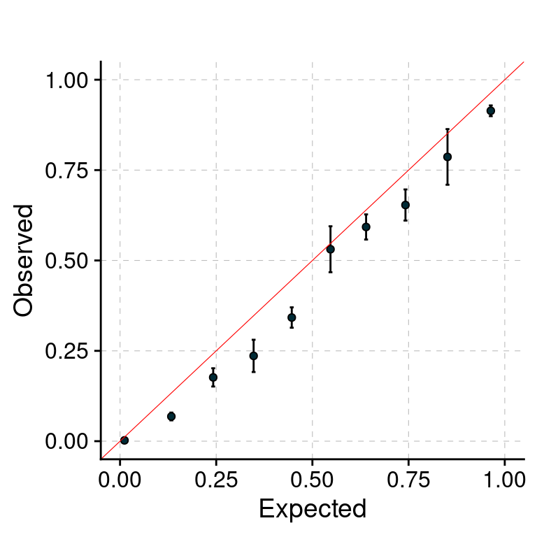
sessionInfo()R version 4.1.0 (2021-05-18)
Platform: x86_64-pc-linux-gnu (64-bit)
Running under: CentOS Linux 7 (Core)
Matrix products: default
BLAS/LAPACK: /software/openblas-0.3.13-el7-x86_64/lib/libopenblas_haswellp-r0.3.13.so
locale:
[1] LC_CTYPE=en_US.UTF-8 LC_NUMERIC=C
[3] LC_TIME=en_US.UTF-8 LC_COLLATE=en_US.UTF-8
[5] LC_MONETARY=en_US.UTF-8 LC_MESSAGES=en_US.UTF-8
[7] LC_PAPER=en_US.UTF-8 LC_NAME=C
[9] LC_ADDRESS=C LC_TELEPHONE=C
[11] LC_MEASUREMENT=en_US.UTF-8 LC_IDENTIFICATION=C
attached base packages:
[1] stats graphics grDevices utils datasets methods base
other attached packages:
[1] plyr_1.8.8 ggpubr_0.6.0 plotrix_3.8-4 cowplot_1.1.1
[5] ggplot2_3.4.0 data.table_1.14.6 ctwas_0.1.40 workflowr_1.7.0
loaded via a namespace (and not attached):
[1] Rcpp_1.0.9 lattice_0.20-44 tidyr_1.3.0 getPass_0.2-2
[5] ps_1.7.2 assertthat_0.2.1 rprojroot_2.0.3 digest_0.6.31
[9] foreach_1.5.2 utf8_1.2.2 R6_2.5.1 backports_1.2.1
[13] evaluate_0.19 highr_0.9 httr_1.4.4 pillar_1.8.1
[17] rlang_1.1.1 rstudioapi_0.14 car_3.1-1 whisker_0.4.1
[21] callr_3.7.3 jquerylib_0.1.4 Matrix_1.3-3 rmarkdown_2.19
[25] labeling_0.4.2 stringr_1.5.0 munsell_0.5.0 broom_1.0.2
[29] compiler_4.1.0 httpuv_1.6.7 xfun_0.35 pkgconfig_2.0.3
[33] htmltools_0.5.4 tidyselect_1.2.0 tibble_3.1.8 logging_0.10-108
[37] codetools_0.2-18 fansi_1.0.3 crayon_1.5.2 dplyr_1.0.10
[41] withr_2.5.0 later_1.3.0 grid_4.1.0 jsonlite_1.8.4
[45] gtable_0.3.1 lifecycle_1.0.3 DBI_1.1.3 git2r_0.30.1
[49] magrittr_2.0.3 scales_1.2.1 carData_3.0-4 cli_3.6.1
[53] stringi_1.7.8 cachem_1.0.6 farver_2.1.0 ggsignif_0.6.4
[57] fs_1.5.2 promises_1.2.0.1 pgenlibr_0.3.2 bslib_0.4.1
[61] vctrs_0.6.3 generics_0.1.3 iterators_1.0.14 tools_4.1.0
[65] glue_1.6.2 purrr_1.0.2 abind_1.4-5 processx_3.8.0
[69] fastmap_1.1.0 yaml_2.3.6 colorspace_2.0-3 rstatix_0.7.2
[73] knitr_1.41 sass_0.4.4