cTWAS paper figures
2025-8-18
Last updated: 2025-09-15
Checks: 6 1
Knit directory: multigroup_ctwas_analysis/
This reproducible R Markdown analysis was created with workflowr (version 1.7.0). The Checks tab describes the reproducibility checks that were applied when the results were created. The Past versions tab lists the development history.
The R Markdown file has unstaged changes. To know which version of
the R Markdown file created these results, you’ll want to first commit
it to the Git repo. If you’re still working on the analysis, you can
ignore this warning. When you’re finished, you can run
wflow_publish to commit the R Markdown file and build the
HTML.
Great job! The global environment was empty. Objects defined in the global environment can affect the analysis in your R Markdown file in unknown ways. For reproduciblity it’s best to always run the code in an empty environment.
The command set.seed(20231112) was run prior to running
the code in the R Markdown file. Setting a seed ensures that any results
that rely on randomness, e.g. subsampling or permutations, are
reproducible.
Great job! Recording the operating system, R version, and package versions is critical for reproducibility.
Nice! There were no cached chunks for this analysis, so you can be confident that you successfully produced the results during this run.
Great job! Using relative paths to the files within your workflowr project makes it easier to run your code on other machines.
Great! You are using Git for version control. Tracking code development and connecting the code version to the results is critical for reproducibility.
The results in this page were generated with repository version f2ff38d. See the Past versions tab to see a history of the changes made to the R Markdown and HTML files.
Note that you need to be careful to ensure that all relevant files for
the analysis have been committed to Git prior to generating the results
(you can use wflow_publish or
wflow_git_commit). workflowr only checks the R Markdown
file, but you know if there are other scripts or data files that it
depends on. Below is the status of the Git repository when the results
were generated:
Unstaged changes:
    Modified:   analysis/ctwas_paper_figures.Rmd
Note that any generated files, e.g. HTML, png, CSS, etc., are not included in this status report because it is ok for generated content to have uncommitted changes.
These are the previous versions of the repository in which changes were
made to the R Markdown (analysis/ctwas_paper_figures.Rmd)
and HTML (docs/ctwas_paper_figures.html) files. If you’ve
configured a remote Git repository (see ?wflow_git_remote),
click on the hyperlinks in the table below to view the files as they
were in that past version.
| File | Version | Author | Date | Message |
|---|---|---|---|---|
| Rmd | f2ff38d | sq-96 | 2025-09-15 | update |
| html | f2ff38d | sq-96 | 2025-09-15 | update |
| Rmd | 6c90f51 | sq-96 | 2025-09-14 | update |
| html | 6c90f51 | sq-96 | 2025-09-14 | update |
| Rmd | cc37918 | sq-96 | 2025-09-14 | update |
| html | cc37918 | sq-96 | 2025-09-14 | update |
| Rmd | 915ef41 | sq-96 | 2025-09-11 | update |
| html | 915ef41 | sq-96 | 2025-09-11 | update |
| Rmd | 07f7145 | sq-96 | 2025-09-11 | update |
| html | 07f7145 | sq-96 | 2025-09-11 | update |
| Rmd | dfd4c68 | sq-96 | 2025-09-11 | update |
| html | dfd4c68 | sq-96 | 2025-09-11 | update |
| Rmd | 95fd6f1 | sq-96 | 2025-09-11 | update |
| html | 74b8361 | sq-96 | 2025-09-07 | update |
| Rmd | c370e05 | sq-96 | 2025-09-05 | update |
| html | c370e05 | sq-96 | 2025-09-05 | update |
| Rmd | 7440fa5 | sq-96 | 2025-09-05 | update |
| html | 7440fa5 | sq-96 | 2025-09-05 | update |
| Rmd | d5606c1 | sq-96 | 2025-09-03 | update |
| html | d5606c1 | sq-96 | 2025-09-03 | update |
| Rmd | 7abbd92 | sq-96 | 2025-08-30 | update |
| html | 7abbd92 | sq-96 | 2025-08-30 | update |
| Rmd | aa1605e | sq-96 | 2025-08-29 | update |
| html | aa1605e | sq-96 | 2025-08-29 | update |
| Rmd | 2273a54 | sq-96 | 2025-08-29 | update |
| html | 2273a54 | sq-96 | 2025-08-29 | update |
| Rmd | 595beb3 | sq-96 | 2025-08-29 | update |
| html | 595beb3 | sq-96 | 2025-08-29 | update |
| Rmd | 4877fe4 | sq-96 | 2025-08-28 | update |
| html | 4877fe4 | sq-96 | 2025-08-28 | update |
| Rmd | c3db7c5 | sq-96 | 2025-08-28 | update |
| html | c3db7c5 | sq-96 | 2025-08-28 | update |
| Rmd | 018ade4 | sq-96 | 2025-08-28 | update |
| html | 018ade4 | sq-96 | 2025-08-28 | update |
| Rmd | b8d0b9c | sq-96 | 2025-08-28 | update |
| html | b8d0b9c | sq-96 | 2025-08-28 | update |
| Rmd | 79c875f | sq-96 | 2025-08-28 | update |
| html | 79c875f | sq-96 | 2025-08-28 | update |
| Rmd | ea08390 | sq-96 | 2025-08-28 | update |
| html | ea08390 | sq-96 | 2025-08-28 | update |
| Rmd | 1c4db8b | sq-96 | 2025-08-28 | update |
| html | 1c4db8b | sq-96 | 2025-08-28 | update |
| Rmd | 7b9b09f | sq-96 | 2025-08-28 | update |
| html | 7b9b09f | sq-96 | 2025-08-28 | update |
| Rmd | 4b9798e | sq-96 | 2025-08-28 | update |
| html | 4b9798e | sq-96 | 2025-08-28 | update |
| Rmd | 81430a0 | sq-96 | 2025-08-28 | update |
| html | 81430a0 | sq-96 | 2025-08-28 | update |
| Rmd | 9633ed7 | sq-96 | 2025-08-22 | update |
| html | 9633ed7 | sq-96 | 2025-08-22 | update |
| Rmd | 609e217 | sq-96 | 2025-08-22 | update |
| html | 609e217 | sq-96 | 2025-08-22 | update |
| Rmd | 6f2a725 | sq-96 | 2025-08-21 | update |
| html | 6f2a725 | sq-96 | 2025-08-21 | update |
| Rmd | 5896c92 | sq-96 | 2025-08-20 | update |
| html | 5896c92 | sq-96 | 2025-08-20 | update |
| Rmd | 4343a9a | sq-96 | 2025-08-20 | update |
| html | 4343a9a | sq-96 | 2025-08-20 | update |
| Rmd | 36913e7 | sq-96 | 2025-08-20 | update |
| html | 36913e7 | sq-96 | 2025-08-20 | update |
| Rmd | 4cdfb66 | sq-96 | 2025-08-20 | update |
| html | 4cdfb66 | sq-96 | 2025-08-20 | update |
| Rmd | b3fe907 | sq-96 | 2025-08-18 | update |
| html | b3fe907 | sq-96 | 2025-08-18 | update |
| Rmd | e41cab7 | sq-96 | 2025-08-18 | update |
| html | e41cab7 | sq-96 | 2025-08-18 | update |
| Rmd | bbd203f | sq-96 | 2025-08-18 | update |
| html | bbd203f | sq-96 | 2025-08-18 | update |
| Rmd | e248888 | sq-96 | 2025-08-18 | update |
| html | e248888 | sq-96 | 2025-08-18 | update |
| Rmd | ee48863 | sq-96 | 2025-08-18 | update |
| html | ee48863 | sq-96 | 2025-08-18 | update |
| Rmd | 6b7c3e2 | sq-96 | 2025-08-18 | update |
| html | 6b7c3e2 | sq-96 | 2025-08-18 | update |
| Rmd | f4bc224 | sq-96 | 2025-08-18 | update |
| html | f4bc224 | sq-96 | 2025-08-18 | update |
| Rmd | fd2ccbd | sq-96 | 2025-08-18 | update |
| html | fd2ccbd | sq-96 | 2025-08-18 | update |
| Rmd | d041eed | sq-96 | 2025-08-18 | update |
| html | d041eed | sq-96 | 2025-08-18 | update |
| Rmd | 3de1191 | sq-96 | 2025-08-18 | update |
| html | 3de1191 | sq-96 | 2025-08-18 | update |
Figure 1: Workflow of M-cTWAS

Figure 2: cTWAS simulations (Correlated Brain Tissues)
Figure 2a: Inflated PHE by single-group analysis
Proportion of heritability explained by gene expression of each
tissue estimated by MESC and cTWAS. cTWAS used pre-trained GTEx v8 gene
expression prediction models from PredictDB. MESC used pre-computed GTEx
v8 gene expression scores. Dashlines show the true PVE value.
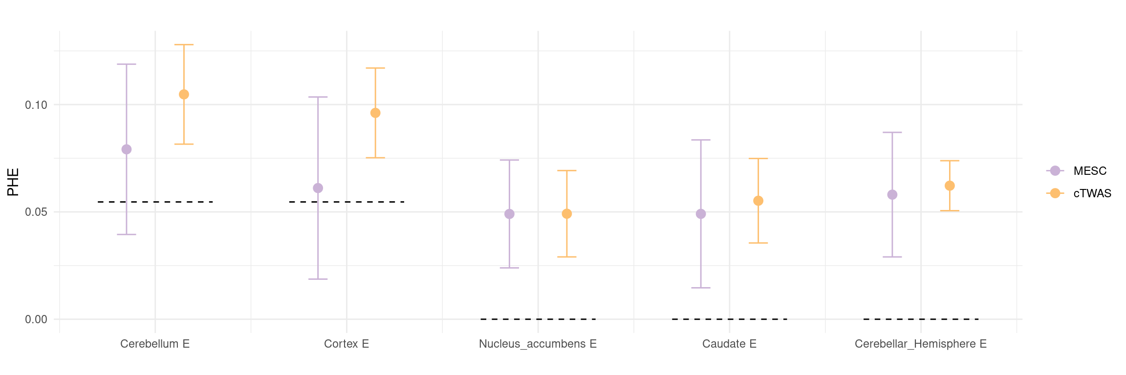
Figure S1: Inflated PHE by single-group analysis
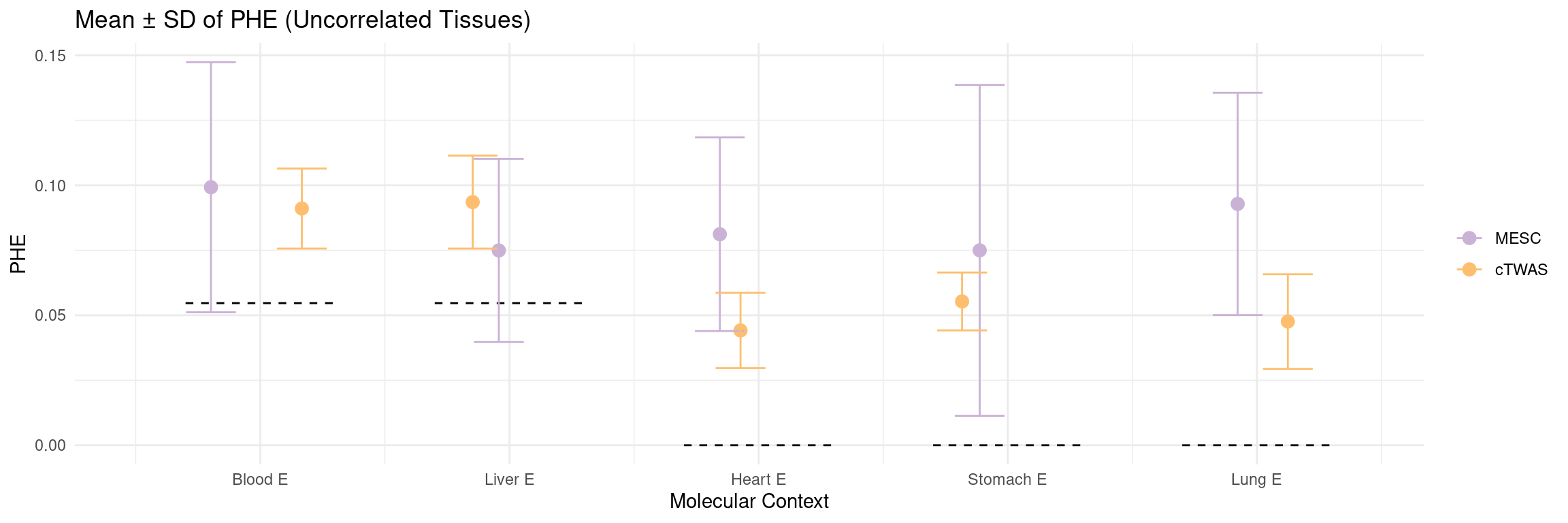
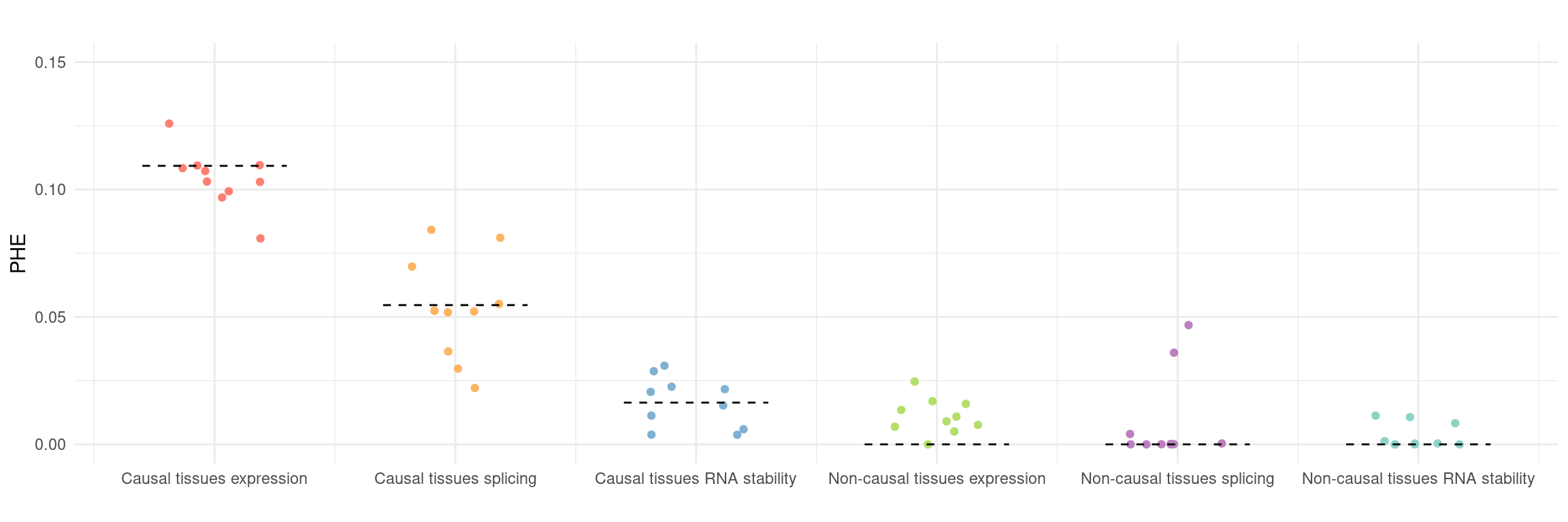
Figure 2b: PHE (correlated tissues)
Proportion of heritability explained by gene expression, splicing and RNA stability of causal and non-causal tissues estimated by M-cTWAS. Causal groups contain two tissues and non-causal groups contain three tissues. Each dot represents one of the ten replicates in simulations. Dashlines show the true PVE value.
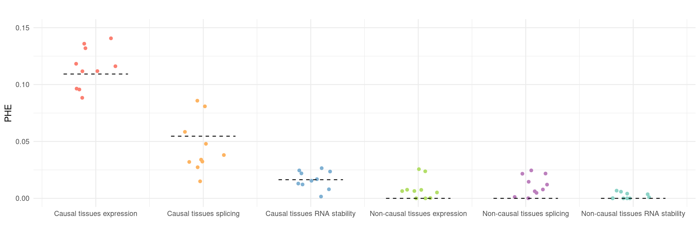
Figure S2: PHE (uncorrelated tissues)
| Version | Author | Date |
|---|---|---|
| 6c90f51 | sq-96 | 2025-09-14 |
| cc37918 | sq-96 | 2025-09-14 |
| dfd4c68 | sq-96 | 2025-09-11 |
| d5606c1 | sq-96 | 2025-09-03 |
| 018ade4 | sq-96 | 2025-08-28 |
| 81430a0 | sq-96 | 2025-08-28 |
| 9633ed7 | sq-96 | 2025-08-22 |
| 6f2a725 | sq-96 | 2025-08-21 |
| 5896c92 | sq-96 | 2025-08-20 |
| 4cdfb66 | sq-96 | 2025-08-20 |
| b3fe907 | sq-96 | 2025-08-18 |
| e41cab7 | sq-96 | 2025-08-18 |
| bbd203f | sq-96 | 2025-08-18 |
Figure S3: Enrichment (correlated and uncorrelated tissues)
Proportion of heritability explained by gene expression, splicing and RNA stability of each tissue estimated by M-cTWAS. Each dot represents one of the ten replicates in simulations. Dashlines show the true PVE value.
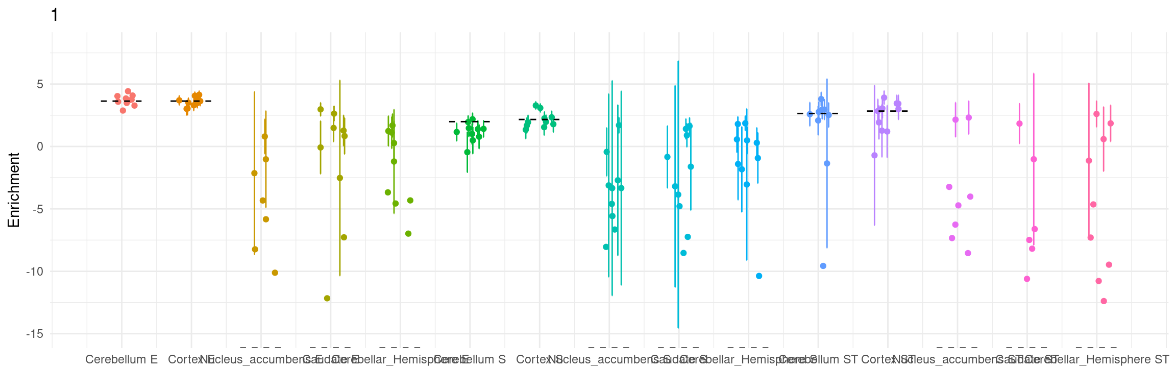
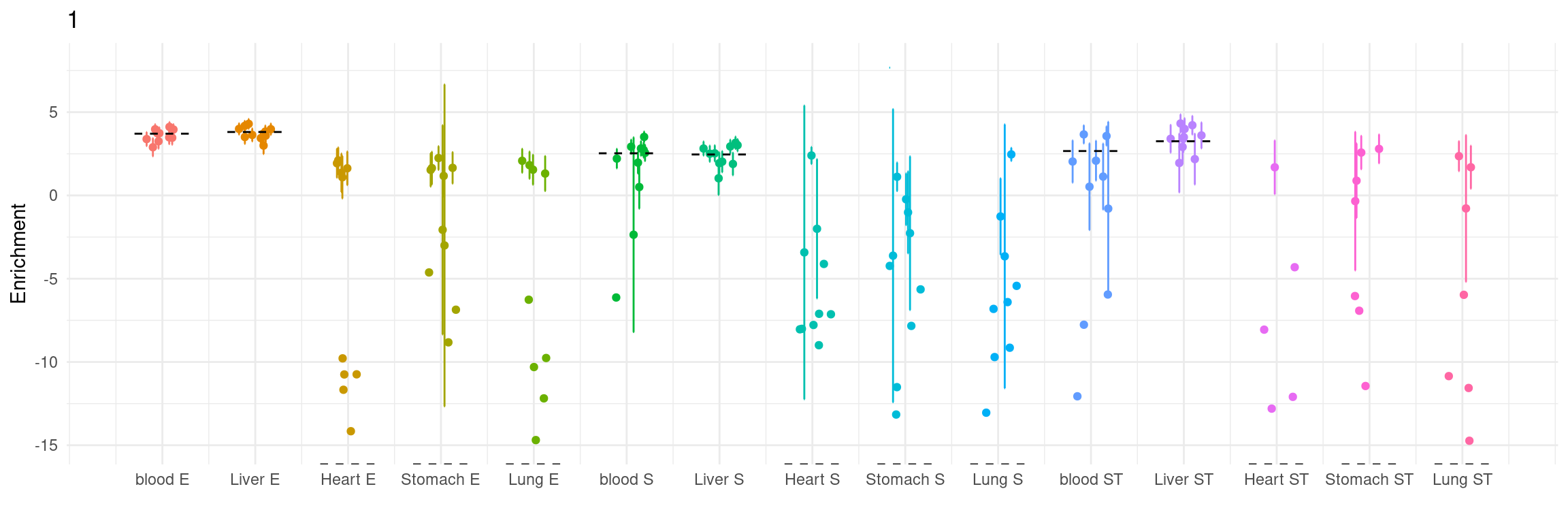
Figure 2c: PIP calibration (correlated)
Gene PIP calibration. Gene PIPs from all simulations are grouped into
bins. The plot shows the proportion of true causal genes (y axis)
against the average PIPs (x axis) under each bin. A well-calibrated
method should produce points along the diagonal lines (red). The ±s.e.
is shown for each point in the vertical bars calculated over ten
independent simulations.
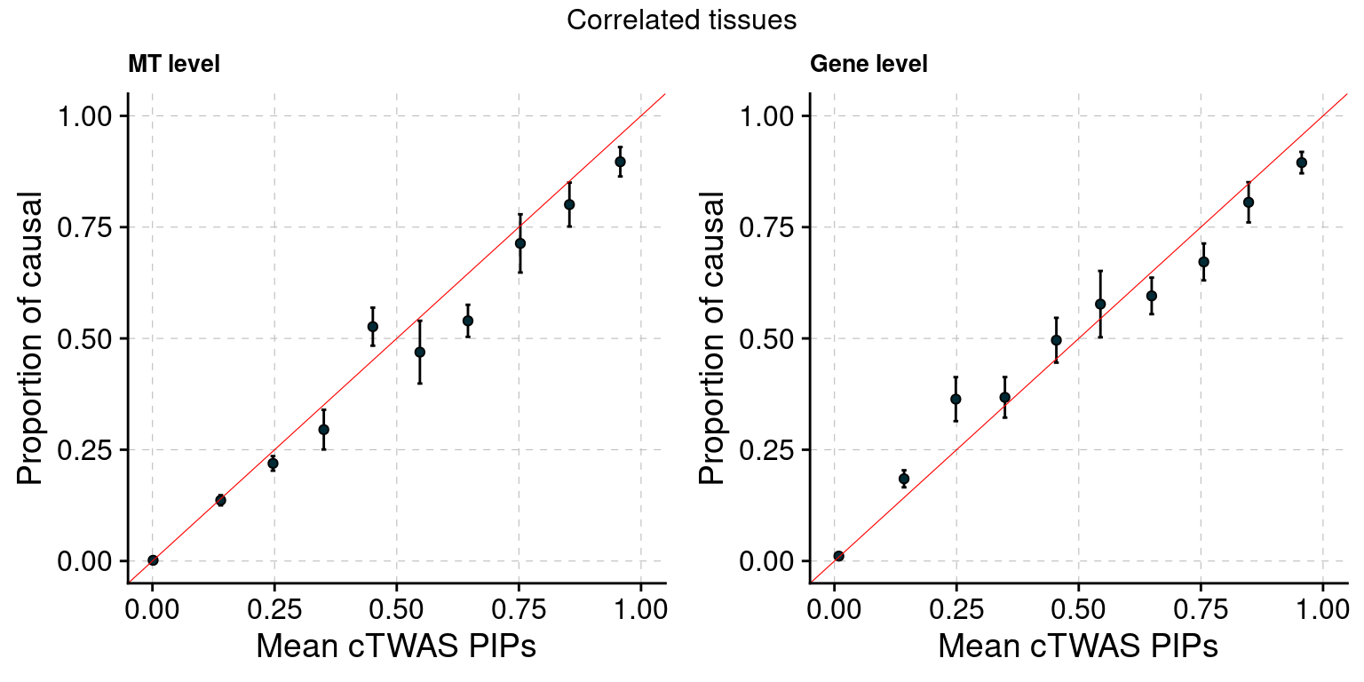
Figure S5: PIP calibration (uncorrelated)
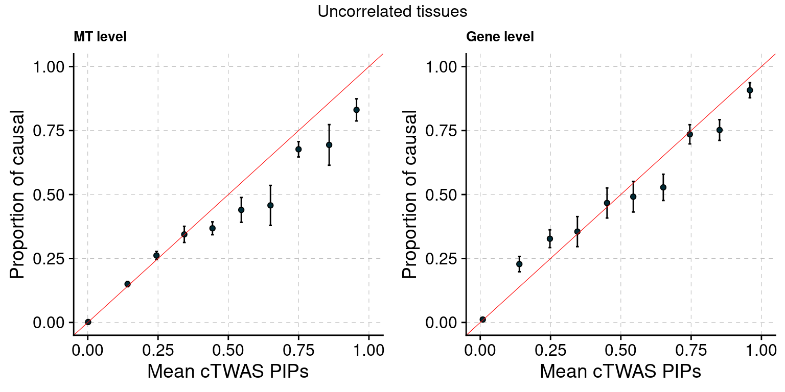
Figure 2d: Power and False discovery rate (correlated)
Number of genes identified by various methods. We used the following
significance thresholds for each method: PIP>0.8 for cTWAS. We use
different colors for causal genes identified by each method, and the top
gray bars indicate noncausal genes. The height of the bar is the mean
over ten independent simulations; the standard error is shown for each
bar in vertical lines from the same ten simulations.
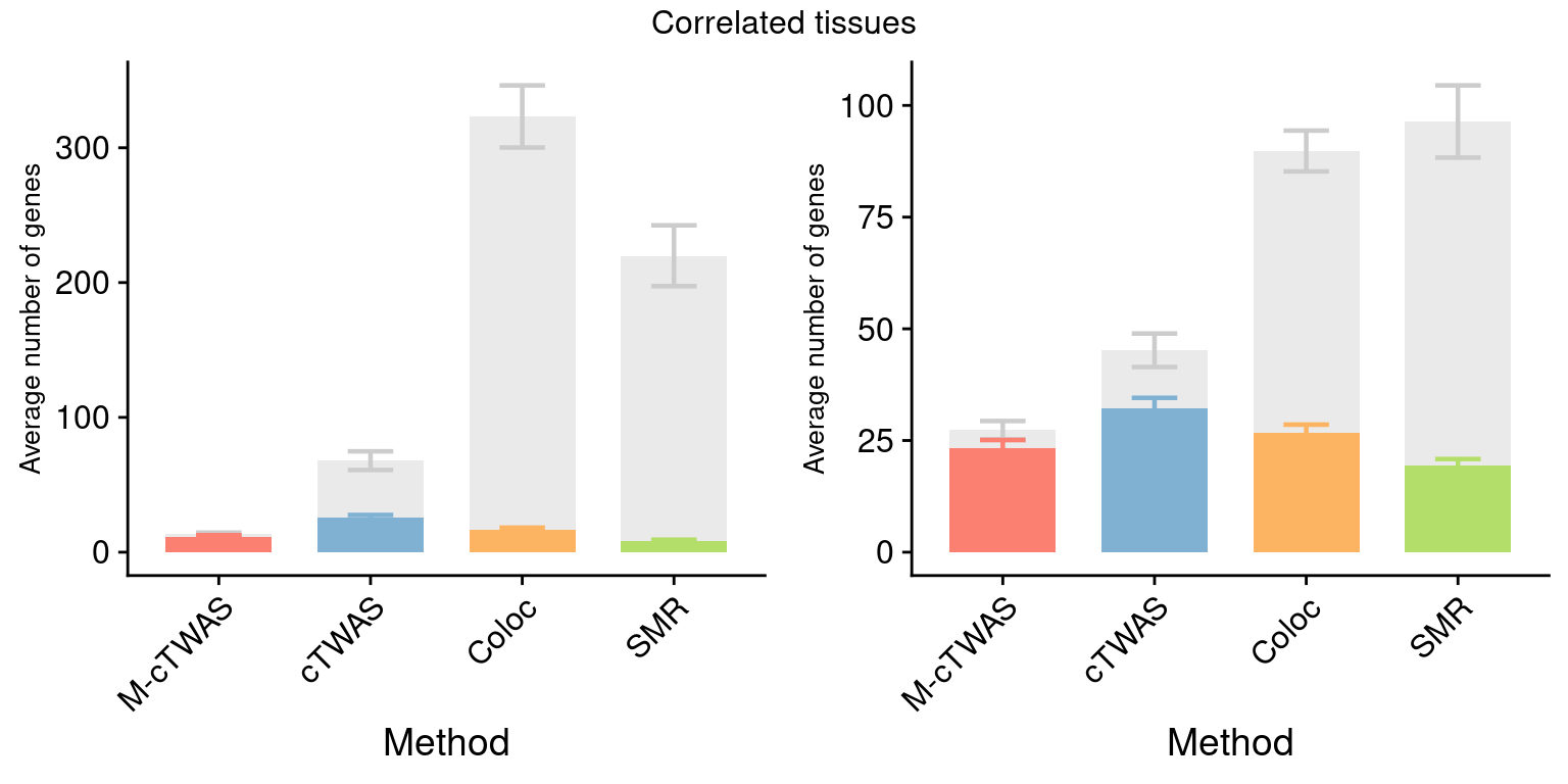
Figure S6: Power and False discovery rate (uncorrelated)
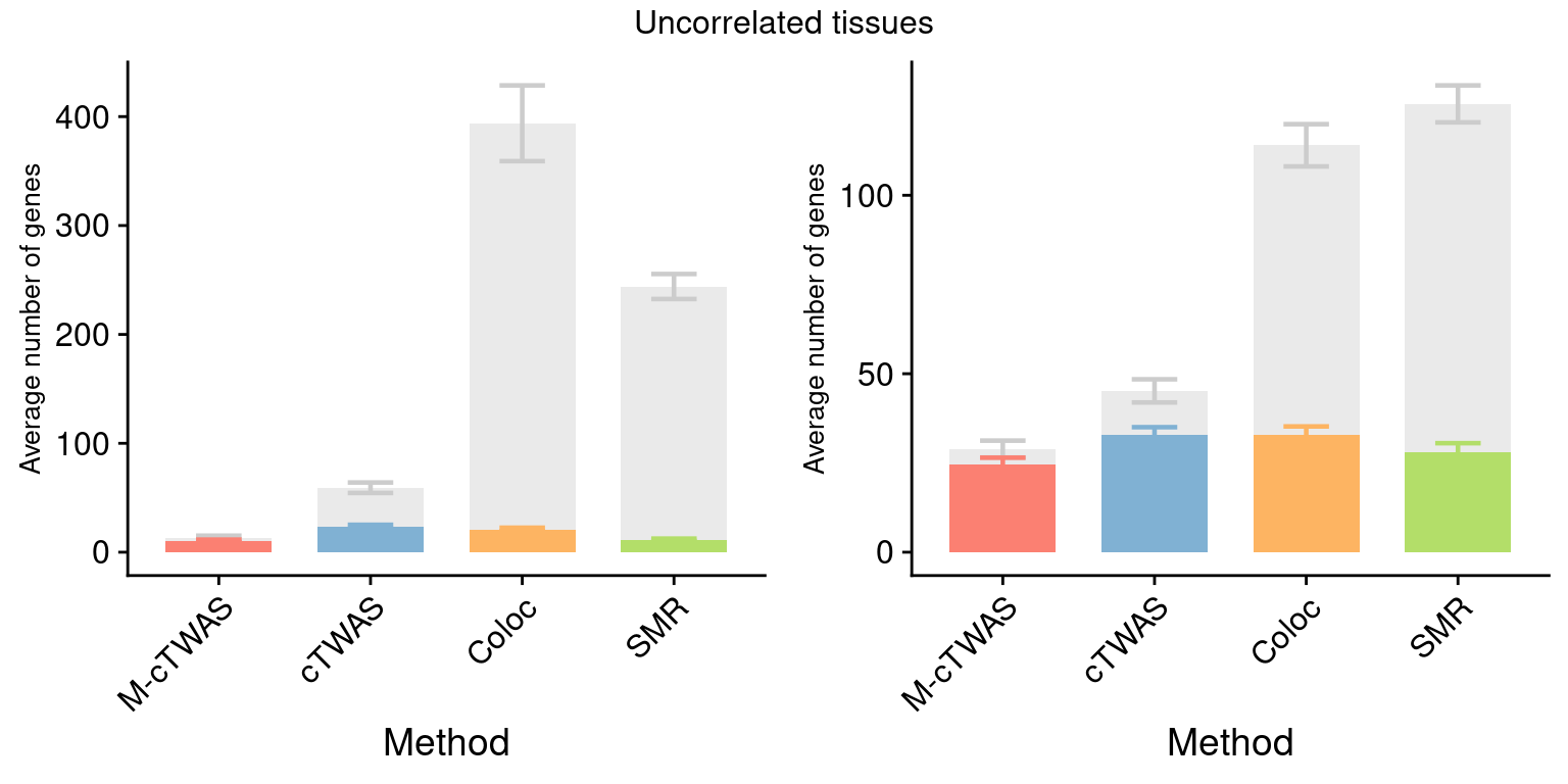
Figure 3: cTWAS estimates genetic architecture of complex traits from GTEx
Figure 3a: Modalities are mostly independent
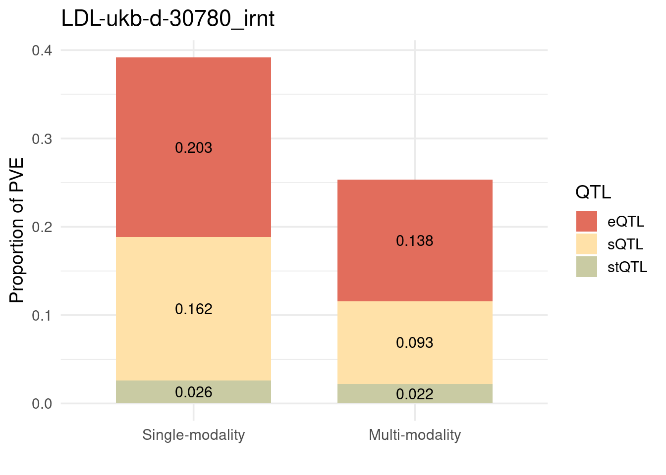
Figure S7: Tissues are often correlated: but one tissue is not enough.
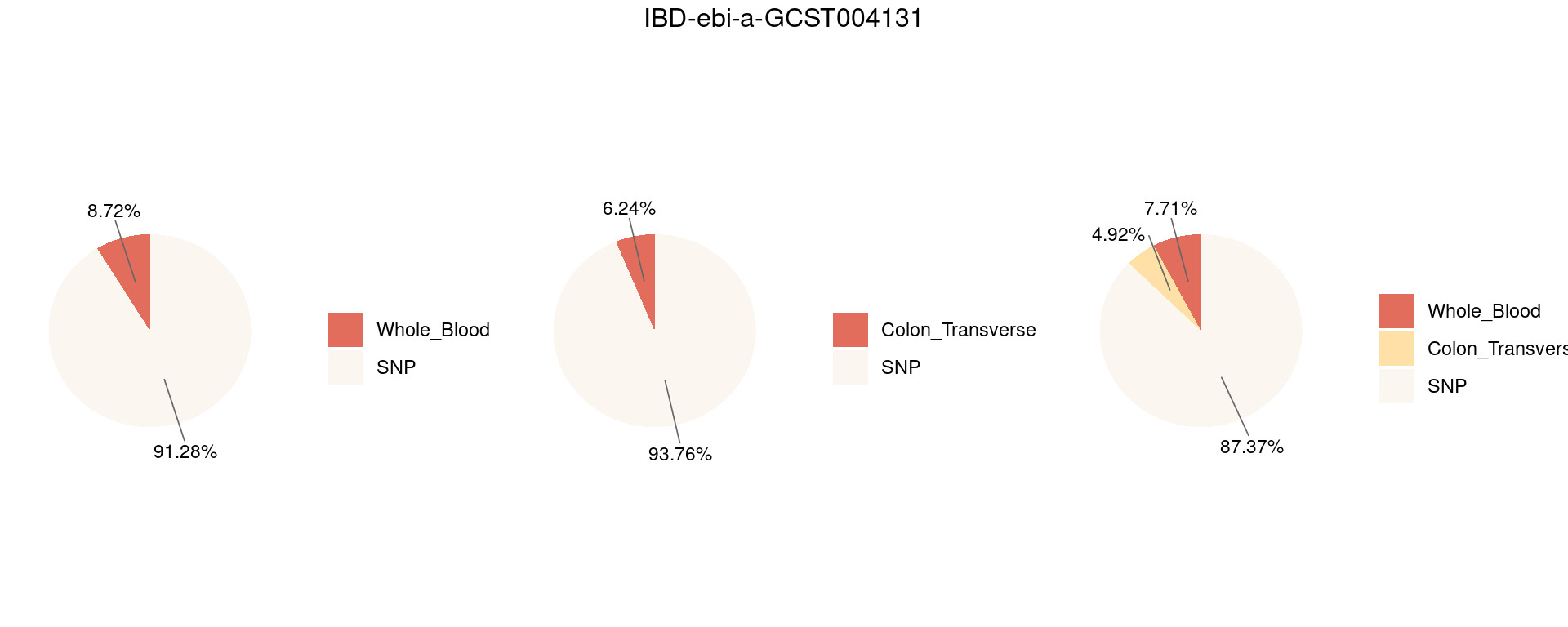
Figure 3b: Shared pattern (eQTL)
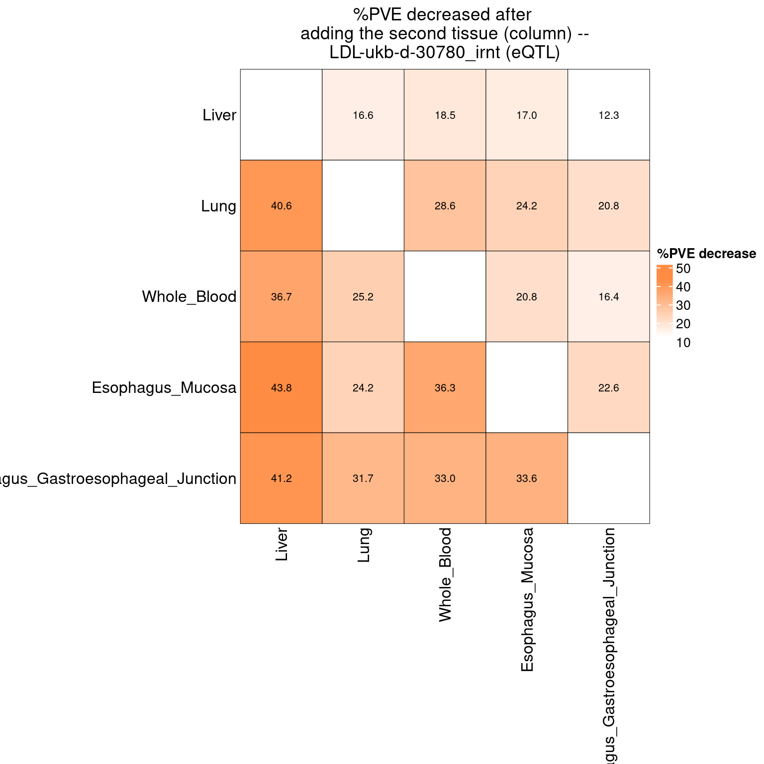
Figure S8: Shared pattern (sQTL)
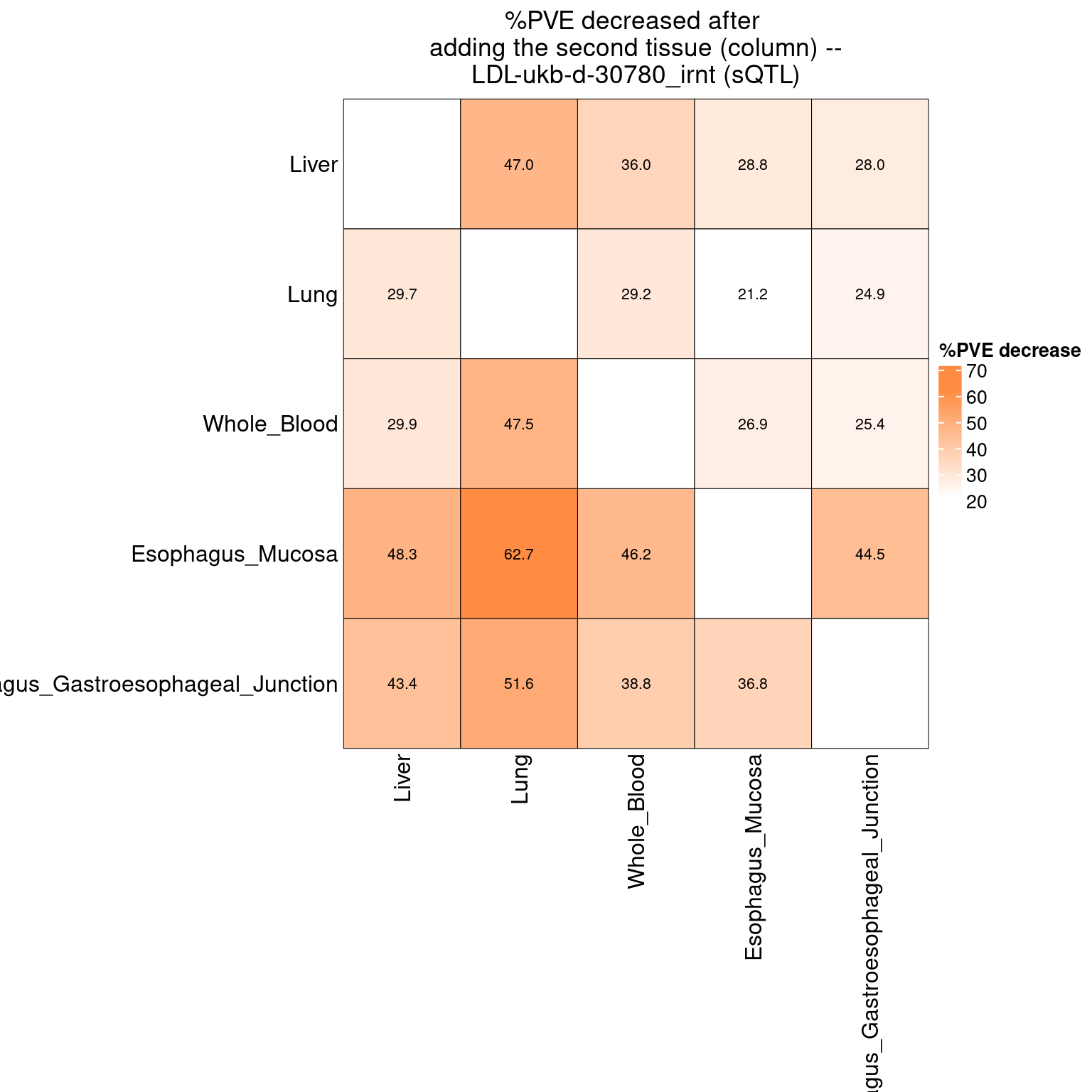
Figure 3c: Partition of h2g (Multiple tissues contribute and Contribution of each modality)
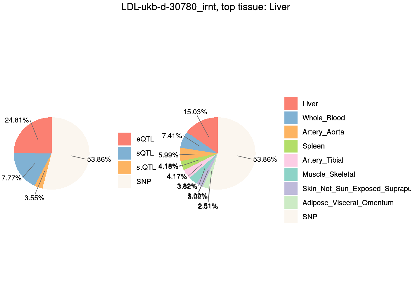
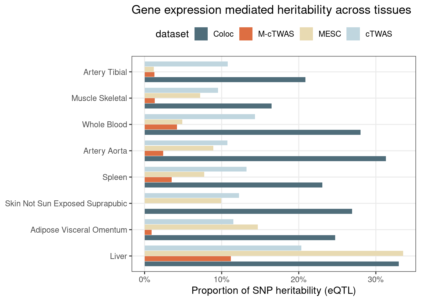
Figure 4: Multi-cTWAS improves the discovery of candidate genes
Figure 4a: Incorporating multiple modality and tissues improves discovery power
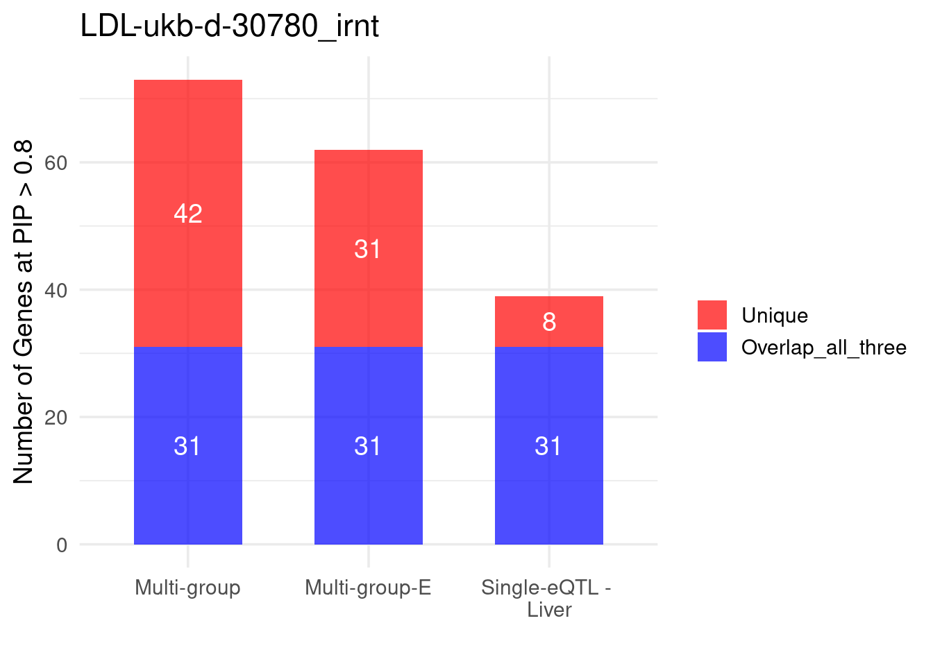
Figure 4b: M-cTWAS identified genes with higher POPS scores
Averaged POPS scores across all traits stratified by M-cTWAS PIPs
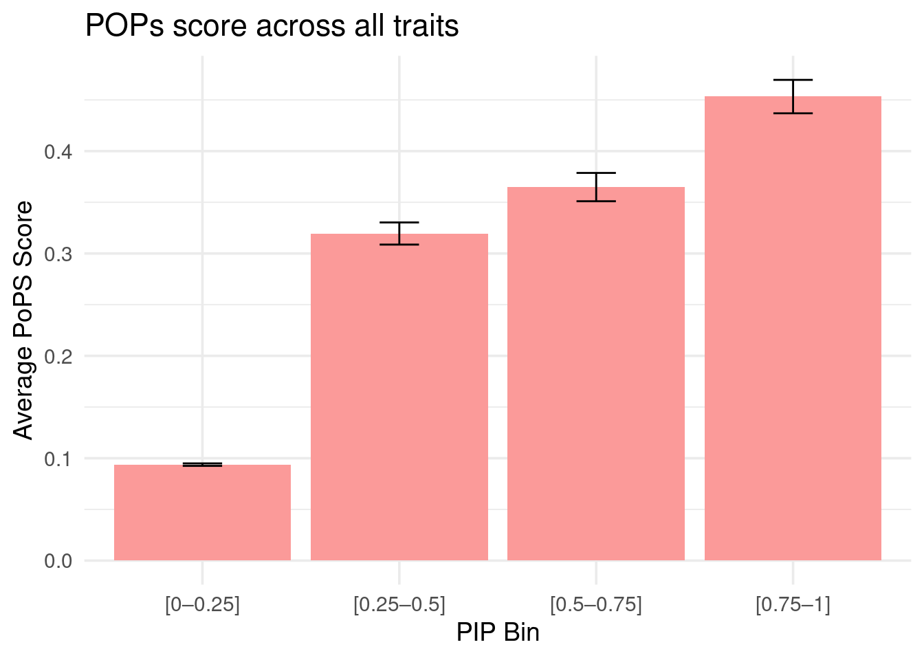
Figure 4c: Validation with Silver Standand Genes
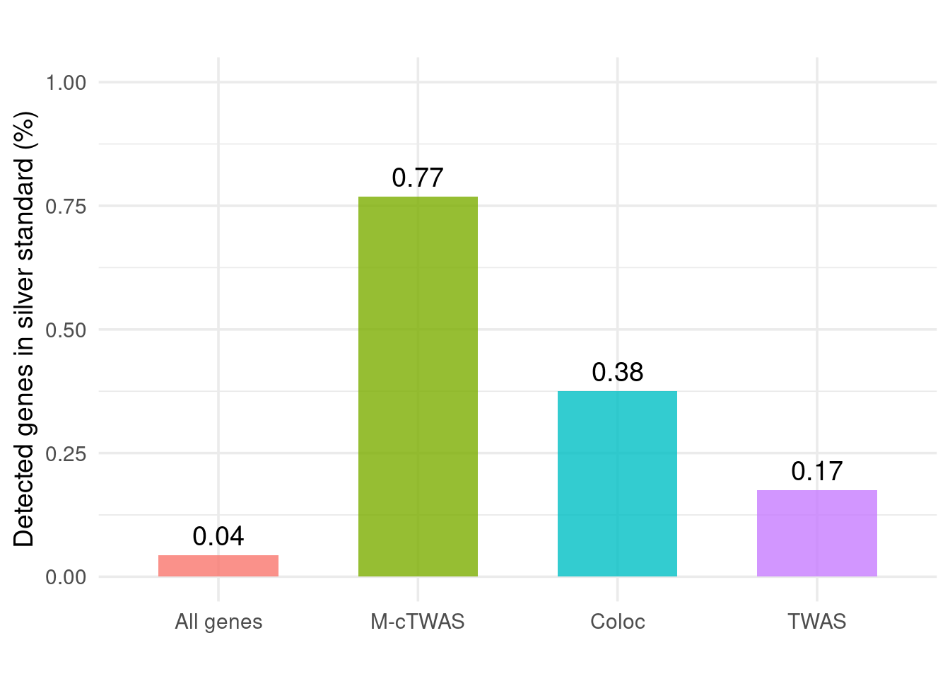
Figure 4d: Comparison of number of signals per region between M-cTWAS, Coloc and TWAS
cTWAS tends to report single genes per locus, while coloc or TWAS report many. The number of signals of Coloc and TWAS are calcuated in regions with TWAS signals (after bonferroni correction). M-cTWAS signals are culated in regions selected by screen region step.
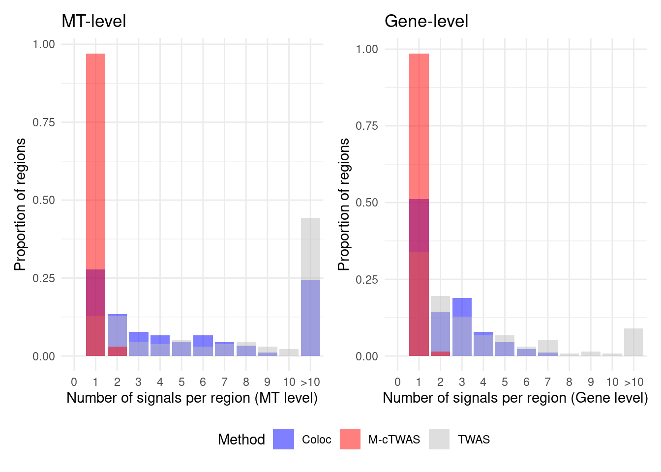
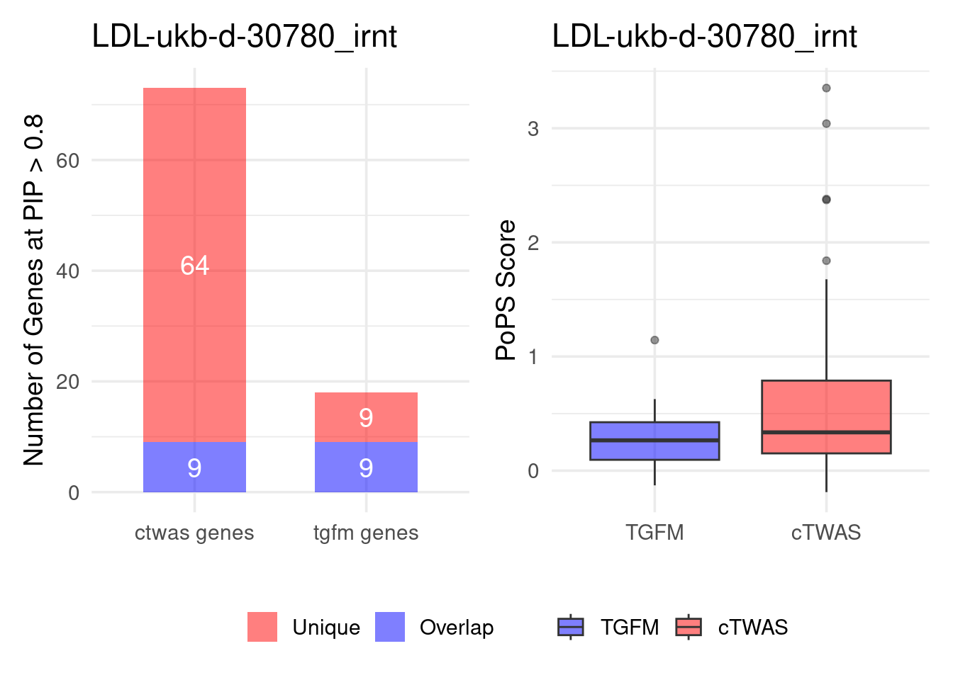
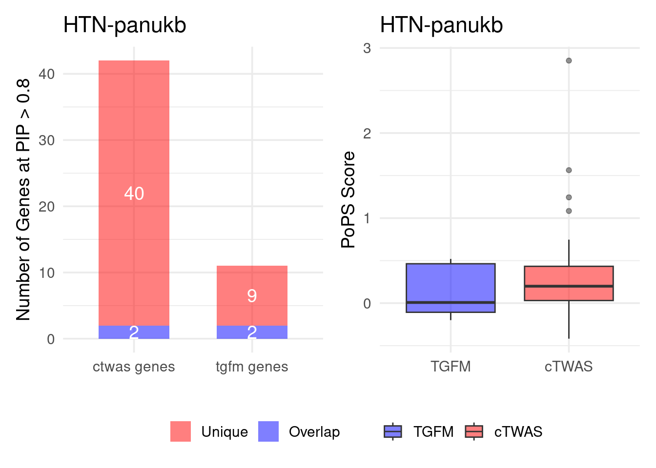
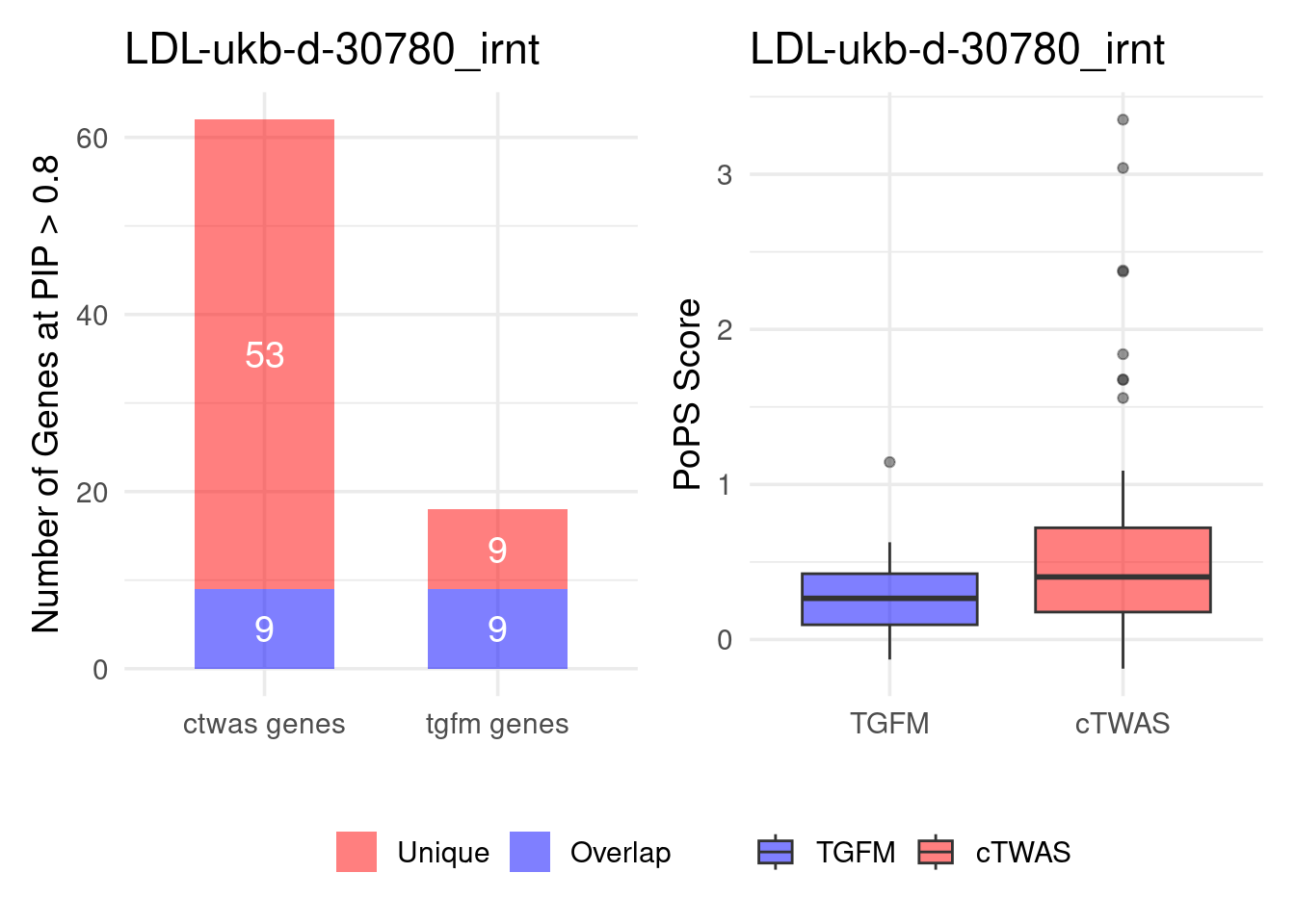
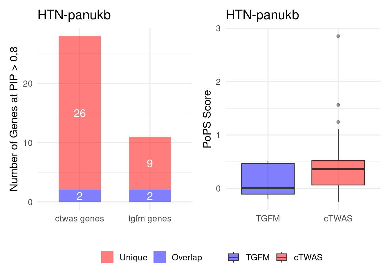
Figure 4e: Compare with TGFM: compare with genes found in the paper. Show that unique genes by cTWAS are valid
For unique genes identified by M-cTWAS and TGFM, I plotted the
distribution of POPS scores and showed that M-cTWAS unique genes have
higher POPS score than TGFM unique genes.
| Version | Author | Date |
|---|---|---|
| 6c90f51 | sq-96 | 2025-09-14 |
| Version | Author | Date |
|---|---|---|
| 6c90f51 | sq-96 | 2025-09-14 |
Figure 5: cTWAS discovers candidate genes for complex traits and provides insights on their molecular mechanisms
Figure 5a: cTWAS helps identify causal modality and context
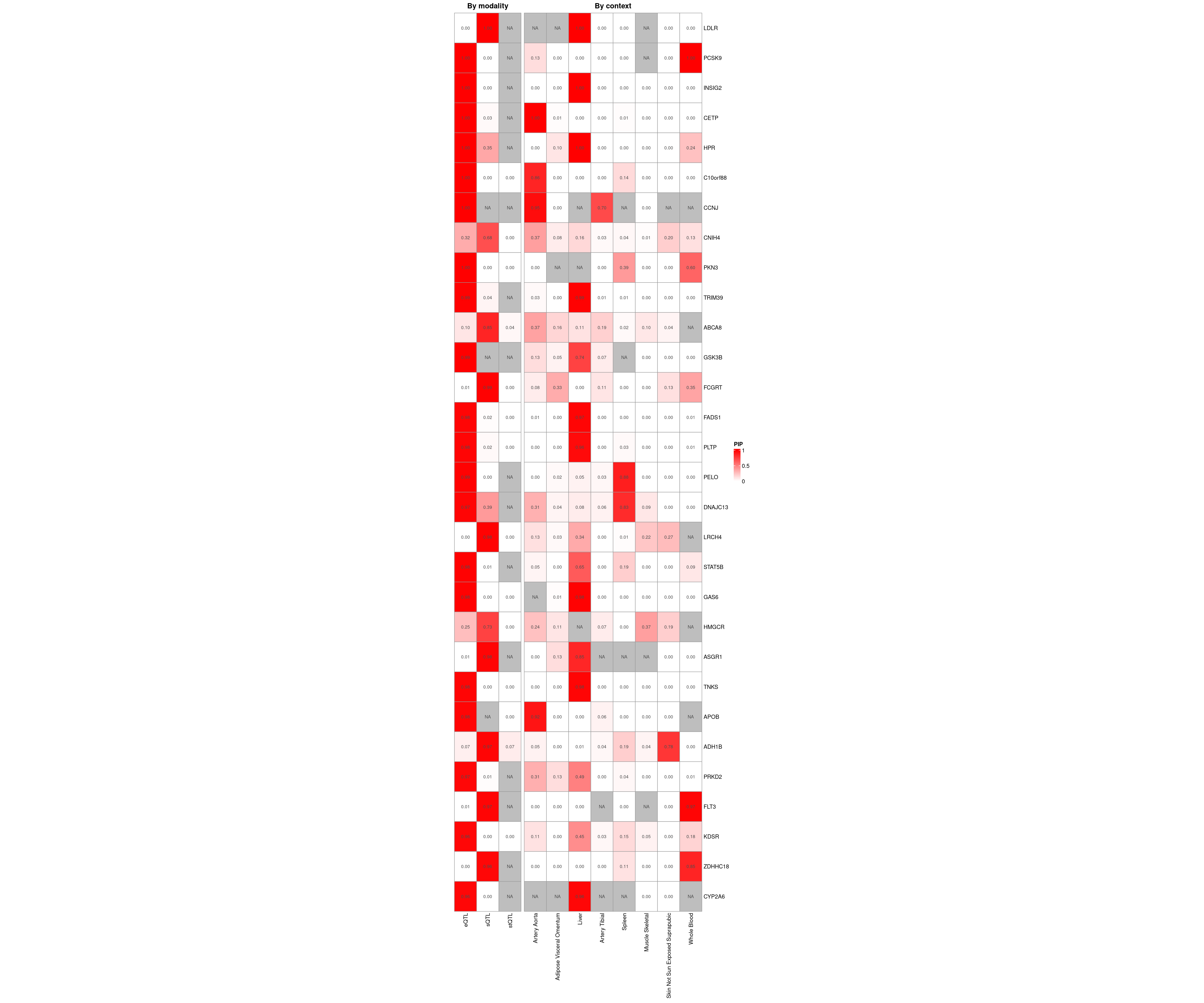
Figure 5b: Gene set enrichment analysis

Figure 5c: Network analysis of candidate genes suggests novel pathways

Figure 5d: A substantial fraction of cTWAS genes are novel
Figure 5e: locus examples

Figure 6: Brain epiQTLs explain a large fraction of missing heritability by eQTLs
Figure 6a: EpiQTLs explain a larger fraction of h2g than eQTLs
| Version | Author | Date |
|---|---|---|
| 6c90f51 | sq-96 | 2025-09-14 |
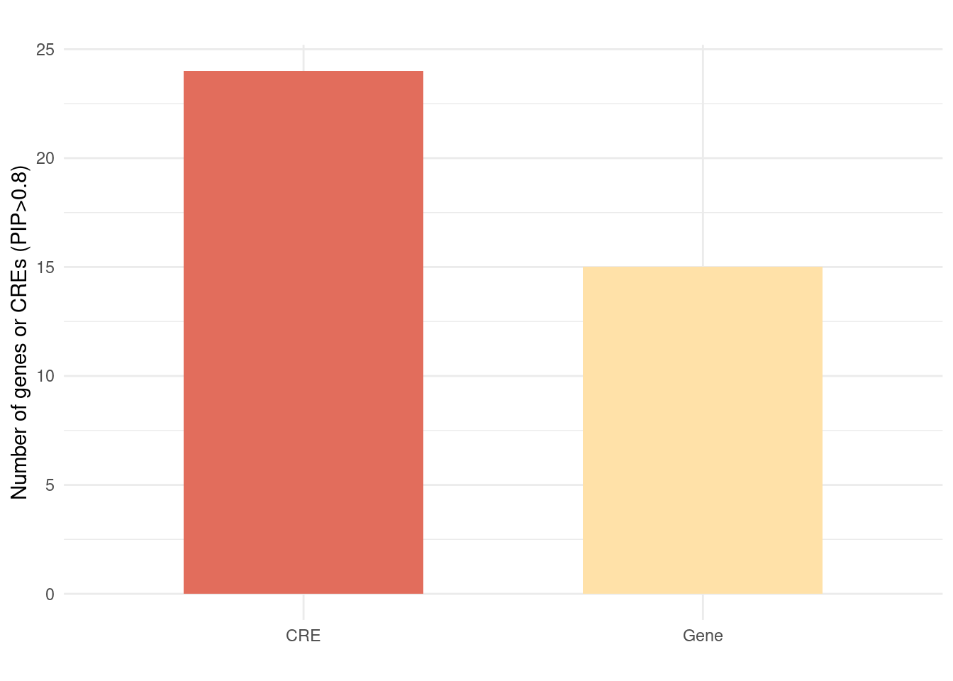
Figure 6b: Using epiQTL discovered novel CREs not explained by eQTLs
| Version | Author | Date |
|---|---|---|
| 6c90f51 | sq-96 | 2025-09-14 |
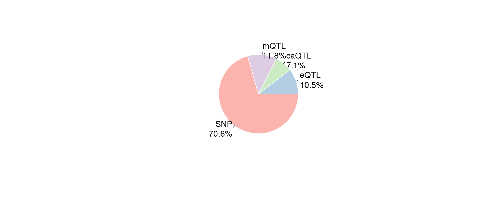
Figure 6c: Validation of meQTL results.
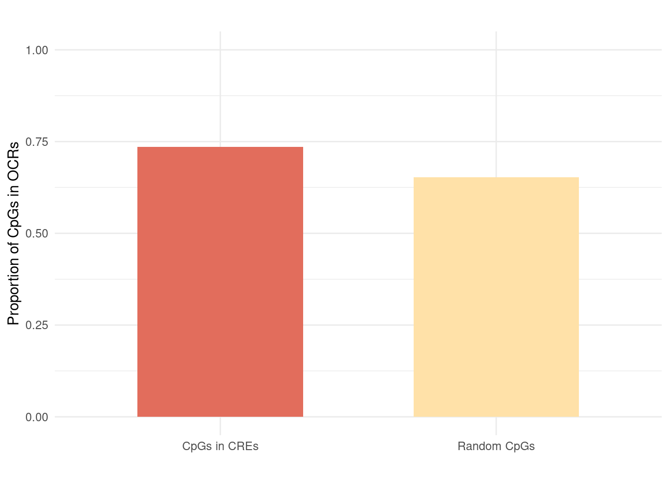
Most randomly sampled CpGs are also in OCRs. Possible reason: Array is designed to measure CpGs near promoter regions.
intergenic
        17
Figure 6d: Do eQTLs explain epiQTLs? Independent PHE
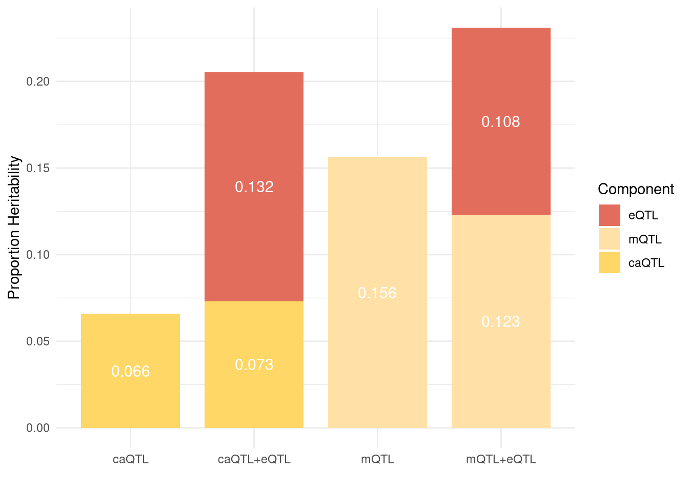
Figure 6e: Do eQTLs explain epiQTLs? few PIPs decreased after adding eQTLs
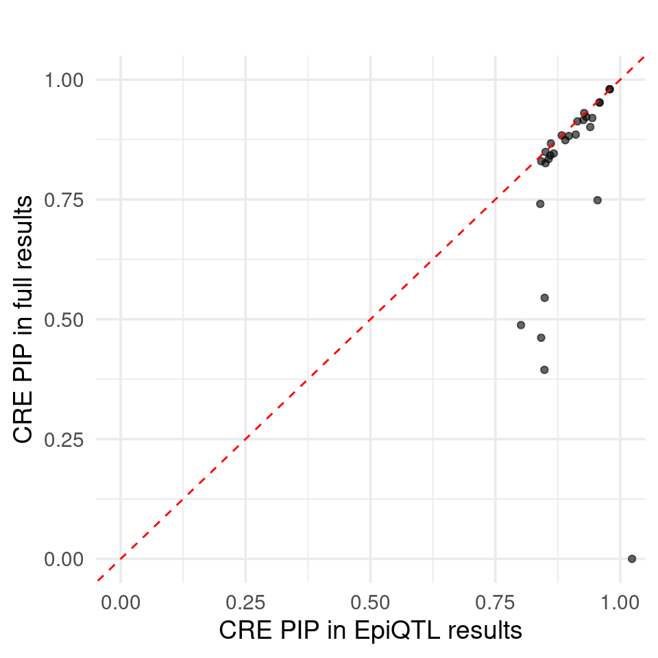
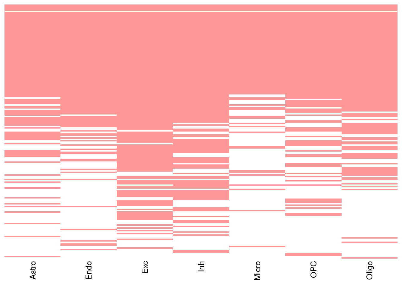
Figure S: Do eQTLs explain epiQTLs? Why eQTLs do not explain epiQTLs. Cell type specific mQTLs
Proportion of CpGs present in exactly k cell-type peaks: peaks n proportion
<int> <int> <num>
1: 1 29 0.16292135
2: 2 20 0.11235955
3: 3 22 0.12359551
4: 4 22 0.12359551
5: 5 10 0.05617978
6: 6 12 0.06741573
7: 7 63 0.35393258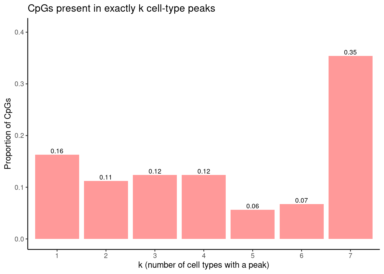
| Version | Author | Date |
|---|---|---|
| 6c90f51 | sq-96 | 2025-09-14 |
Figure S: Do eQTLs explain epiQTLs? GTEx is limited in power. Most mQTLs and caQTLs are eQTLs in MetaBrain eQTL
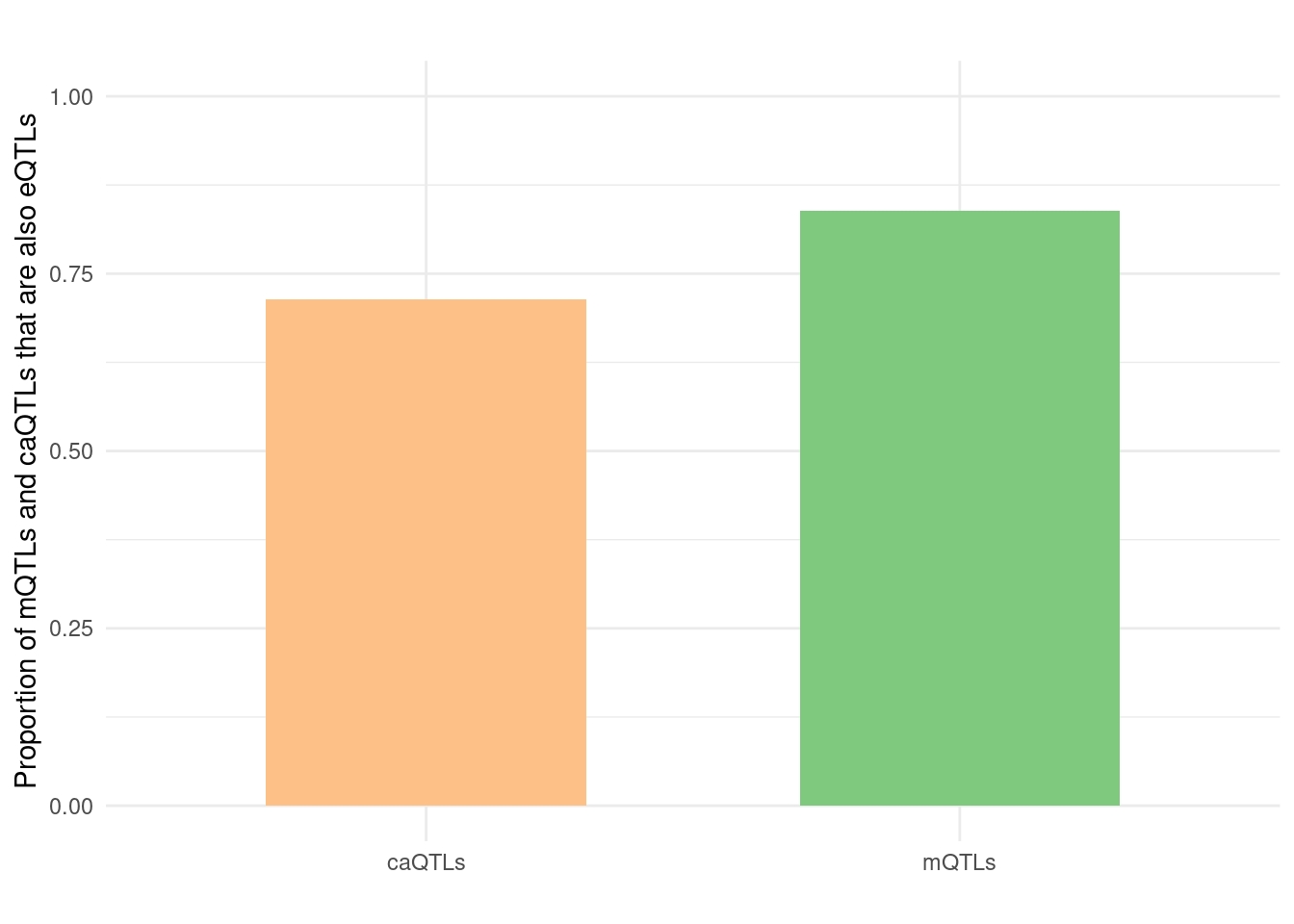
Figure 6d: Do epiQTLs explain eqtlS? Independent PHE
param_eQTL <- readRDS("/project2/xinhe/shengqian/cTWAS_epigenetics/results/SCZ_eQTL/SCZ_eQTL.parameters.RDS")
param_eQTL_epiQTL <- readRDS("/project2/xinhe/shengqian/cTWAS_epigenetics/results/SCZ_eQTL_caQTL_mQTL/SCZ_eQTL_caQTL_mQTL.parameters.RDS")

# Extract values from your objects
bar1_eQTL <- sum(param_eQTL$prop_heritability[1:5])

bar2_eQTL <- sum(param_eQTL_epiQTL$prop_heritability[1:5])
bar2_epi <- sum(param_eQTL_epiQTL$prop_heritability[6:8])

# Data
df2 <- data.frame(
  Bar = c("eQTL", "eQTL+epiQTL", "eQTL+epiQTL"),
  Component = c("eQTL", "eQTL", "epiQTL"),
  Value = c(bar1_eQTL, bar2_eQTL, bar2_epi)
)

# 1) Put eQTL first in levels (bottom of stack)
df2$Component <- factor(df2$Component, levels = c("epiQTL", "eQTL"))

ggplot(df2, aes(x = Bar, y = Value, fill = Component)) +
  # 2) Explicitly keep default (non-reversed) stacking
  geom_bar(stat = "identity", position = position_stack(reverse = FALSE), width = 0.6) +
  geom_text(aes(label = round(Value, 3)),
            position = position_stack(vjust = 0.5, reverse = FALSE),
            color = "white", size = 4) +
  scale_fill_manual(values = c("eQTL" = "#ffe1a8", "epiQTL" = "#e26d5c"),
                    breaks = c("eQTL", "epiQTL")) +
  theme_minimal() +
  labs(y = "Proportion Heritability", x = "", fill = "Component")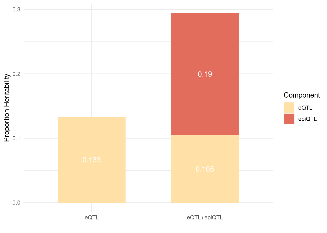
| Version | Author | Date |
|---|---|---|
| 6c90f51 | sq-96 | 2025-09-14 |
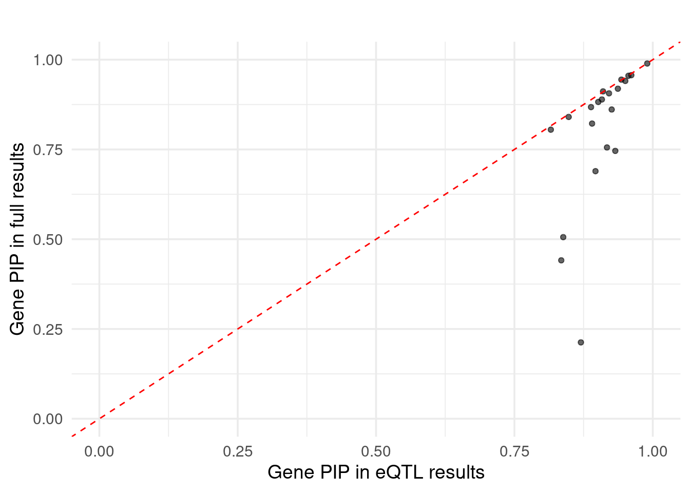
Figure 6d: Do epiQTLs explain eqtlS? few PIPs decreased aftering adding epiQTLs
| Version | Author | Date |
|---|---|---|
| 6c90f51 | sq-96 | 2025-09-14 |
sessionInfo()R version 4.2.0 (2022-04-22)
Platform: x86_64-pc-linux-gnu (64-bit)
Running under: CentOS Linux 7 (Core)
Matrix products: default
BLAS/LAPACK: /software/openblas-0.3.13-el7-x86_64/lib/libopenblas_haswellp-r0.3.13.so
locale:
[1] LC_CTYPE=en_US.UTF-8 LC_NUMERIC=C LC_TIME=C
[4] LC_COLLATE=C LC_MONETARY=C LC_MESSAGES=C
[7] LC_PAPER=C LC_NAME=C LC_ADDRESS=C
[10] LC_TELEPHONE=C LC_MEASUREMENT=C LC_IDENTIFICATION=C
attached base packages:
[1] stats4 grid stats graphics grDevices utils datasets
[8] methods base
other attached packages:
[1] grex_1.9 patchwork_1.3.0
[3] circlize_0.4.15 plotrix_3.8-2
[5] cowplot_1.1.3 ggpubr_0.6.0
[7] scales_1.3.0 RColorBrewer_1.1-3
[9] RSQLite_2.3.7 mapgen_0.5.12
[11] ComplexHeatmap_2.12.0 EnsDb.Hsapiens.v86_2.99.0
[13] ensembldb_2.22.0 AnnotationFilter_1.22.0
[15] GenomicFeatures_1.50.4 AnnotationDbi_1.60.2
[17] Biobase_2.58.0 GenomicRanges_1.50.2
[19] GenomeInfoDb_1.34.9 IRanges_2.32.0
[21] S4Vectors_0.36.2 BiocGenerics_0.44.0
[23] pheatmap_1.0.12 dplyr_1.1.4
[25] egg_0.4.5 gridExtra_2.3
[27] ggrepel_0.9.6 ggplot2_3.5.1
[29] data.table_1.16.0 ctwas_0.5.32
[31] workflowr_1.7.0
loaded via a namespace (and not attached):
[1] backports_1.4.1 BiocFileCache_2.6.1
[3] plyr_1.8.7 repr_1.1.4
[5] lazyeval_0.2.2 BiocParallel_1.32.6
[7] LDlinkR_1.4.0 digest_0.6.37
[9] foreach_1.5.2 htmltools_0.5.8.1
[11] fansi_1.0.6 magrittr_2.0.3
[13] memoise_2.0.1 cluster_2.1.3
[15] doParallel_1.0.17 tzdb_0.4.0
[17] Biostrings_2.66.0 readr_2.1.5
[19] AMR_2.1.1 matrixStats_1.4.1
[21] locuszoomr_0.3.5 prettyunits_1.2.0
[23] colorspace_2.1-1 skimr_2.1.4
[25] blob_1.2.4 rappdirs_0.3.3
[27] xfun_0.47 callr_3.7.2
[29] crayon_1.5.3 RCurl_1.98-1.16
[31] jsonlite_1.8.9 zoo_1.8-12
[33] iterators_1.0.14 glue_1.7.0
[35] gtable_0.3.5 zlibbioc_1.44.0
[37] XVector_0.38.0 GetoptLong_1.0.5
[39] DelayedArray_0.24.0 car_3.1-1
[41] shape_1.4.6 abind_1.4-5
[43] DBI_1.2.3 rstatix_0.7.2
[45] Rcpp_1.0.13 viridisLite_0.4.2
[47] progress_1.2.3 clue_0.3-61
[49] bit_4.5.0 htmlwidgets_1.6.4
[51] httr_1.4.7 farver_2.1.2
[53] reshape_0.8.9 pkgconfig_2.0.3
[55] XML_3.99-0.14 sass_0.4.9
[57] dbplyr_2.5.0 utf8_1.2.4
[59] labeling_0.4.3 tidyselect_1.2.1
[61] rlang_1.1.4 later_1.3.2
[63] munsell_0.5.1 pgenlibr_0.3.7
[65] tools_4.2.0 cachem_1.1.0
[67] cli_3.6.3 generics_0.1.3
[69] broom_1.0.5 evaluate_1.0.0
[71] stringr_1.5.1 fastmap_1.2.0
[73] yaml_2.3.10 processx_3.7.0
[75] knitr_1.48 bit64_4.5.2
[77] fs_1.6.4 purrr_1.0.2
[79] KEGGREST_1.38.0 whisker_0.4
[81] xml2_1.3.3 biomaRt_2.54.1
[83] compiler_4.2.0 rstudioapi_0.14
[85] susieR_0.12.35 plotly_4.10.4
[87] filelock_1.0.3 curl_5.2.3
[89] png_0.1-7 ggsignif_0.6.3
[91] tibble_3.2.1 bslib_0.8.0
[93] stringi_1.8.4 highr_0.11
[95] ps_1.7.1 lattice_0.20-45
[97] ProtGenerics_1.30.0 Matrix_1.5-3
[99] vctrs_0.6.5 pillar_1.9.0
[101] lifecycle_1.0.4 jquerylib_0.1.4
[103] GlobalOptions_0.1.2 bitops_1.0-8
[105] irlba_2.3.5.1 httpuv_1.6.5
[107] rtracklayer_1.58.0 R6_2.6.1
[109] BiocIO_1.8.0 promises_1.3.0
[111] codetools_0.2-18 SummarizedExperiment_1.28.0
[113] rprojroot_2.0.3 rjson_0.2.23
[115] withr_3.0.1 GenomicAlignments_1.34.1
[117] Rsamtools_2.14.0 GenomeInfoDbData_1.2.9
[119] parallel_4.2.0 hms_1.1.3
[121] tidyverse_2.0.0 tidyr_1.3.1
[123] gggrid_0.2-0 rmarkdown_2.28
[125] carData_3.0-5 MatrixGenerics_1.10.0
[127] Cairo_1.6-0 logging_0.10-108
[129] git2r_0.30.1 mixsqp_0.3-54
[131] getPass_0.2-2 base64enc_0.1-3
[133] restfulr_0.0.15