6 Traits, 5 tissues, eQTL + sQTL + apaQTL – compute ukbb LD, weights are from Munro et al
XSun
2024-05-27
Last updated: 2024-06-13
Checks: 6 1
Knit directory: multigroup_ctwas_analysis/
This reproducible R Markdown analysis was created with workflowr (version 1.7.0). The Checks tab describes the reproducibility checks that were applied when the results were created. The Past versions tab lists the development history.
The R Markdown is untracked by Git. To know which version of the R
Markdown file created these results, you’ll want to first commit it to
the Git repo. If you’re still working on the analysis, you can ignore
this warning. When you’re finished, you can run
wflow_publish to commit the R Markdown file and build the
HTML.
Great job! The global environment was empty. Objects defined in the global environment can affect the analysis in your R Markdown file in unknown ways. For reproduciblity it’s best to always run the code in an empty environment.
The command set.seed(20231112) was run prior to running
the code in the R Markdown file. Setting a seed ensures that any results
that rely on randomness, e.g. subsampling or permutations, are
reproducible.
Great job! Recording the operating system, R version, and package versions is critical for reproducibility.
Nice! There were no cached chunks for this analysis, so you can be confident that you successfully produced the results during this run.
Great job! Using relative paths to the files within your workflowr project makes it easier to run your code on other machines.
Great! You are using Git for version control. Tracking code development and connecting the code version to the results is critical for reproducibility.
The results in this page were generated with repository version f82f6b4. See the Past versions tab to see a history of the changes made to the R Markdown and HTML files.
Note that you need to be careful to ensure that all relevant files for
the analysis have been committed to Git prior to generating the results
(you can use wflow_publish or
wflow_git_commit). workflowr only checks the R Markdown
file, but you know if there are other scripts or data files that it
depends on. Below is the status of the Git repository when the results
were generated:
Ignored files:
    Ignored:    .Rhistory
    Ignored:    results/

Untracked files:
    Untracked:  analysis/multi_group_6traits_15weights_ukbb_munro.Rmd

Unstaged changes:
    Modified:   analysis/index.Rmd
    Modified:   analysis/multi_group_6traits_15weights_ukbb.Rmd
Note that any generated files, e.g. HTML, png, CSS, etc., are not included in this status report because it is ok for generated content to have uncommitted changes.
There are no past versions. Publish this analysis with
wflow_publish() to start tracking its development.
Overview
Tissues
The independent tissues are selected by single tissue analysis
Omics
eQTL, sQTL, apaQTL weights are from Munro et al.
Settings
- Weight processing:
PredictDB:
all the PredictDB are converted from FUSION weights
- drop_strand_ambig = TRUE,
- scale_by_ld_variance = F (FUSION converted weights)
- load_predictdb_LD = F,
- Parameter estimation and fine-mapping
- niter_prefit = 5,
- niter = 60,
- L = 3,
- group_prior_var_structure = “shared_type”,
- maxSNP = 20000,
- min_nonSNP_PIP = 0.5,
- Memory requested
- cpus-per-task=2
- mem=200G
over 30h running time
Results
Results from multi-group analysis
The results are summarized by
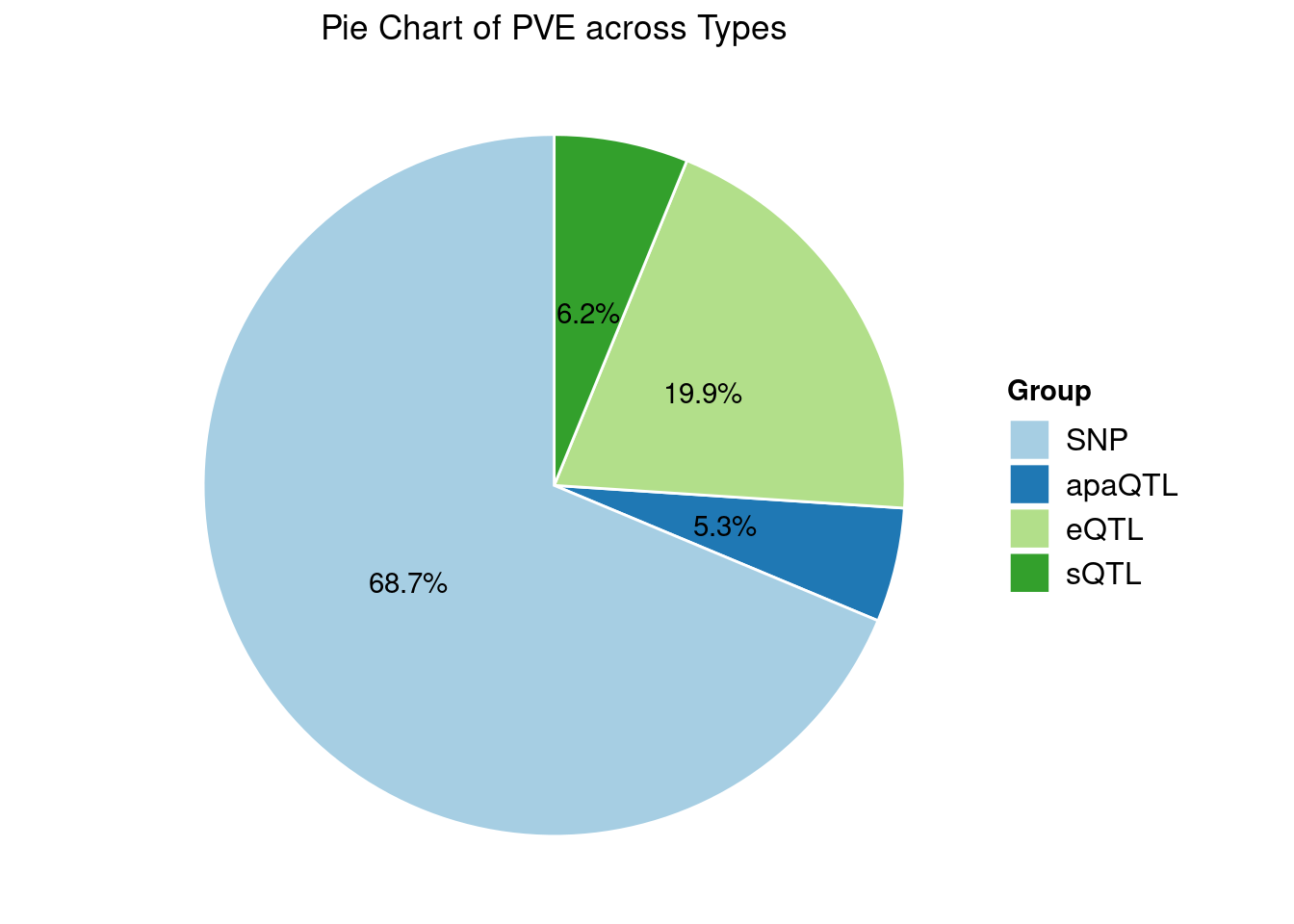
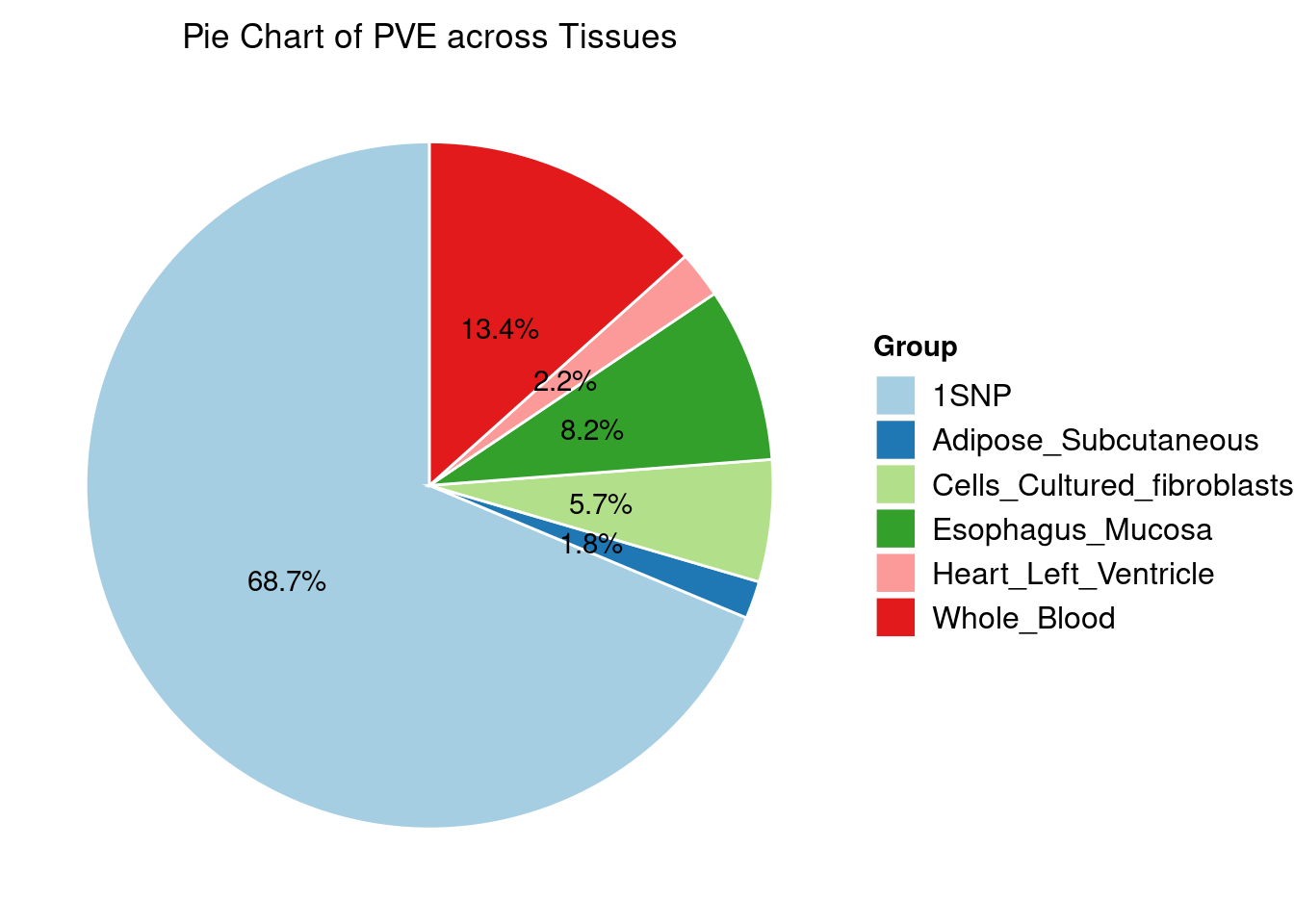
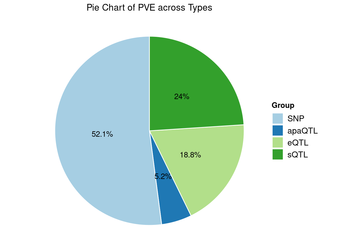
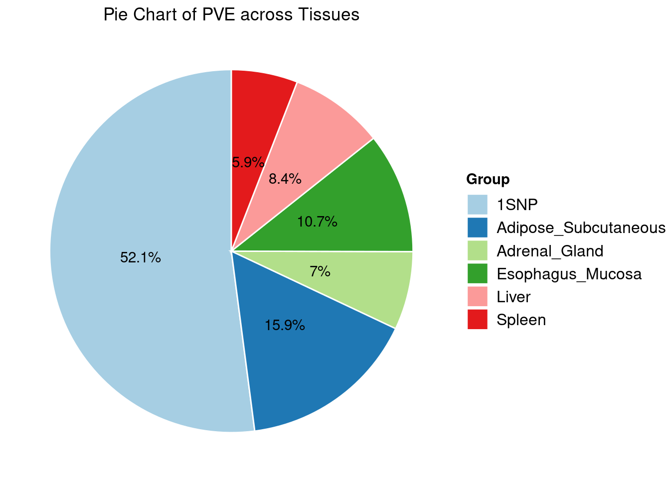
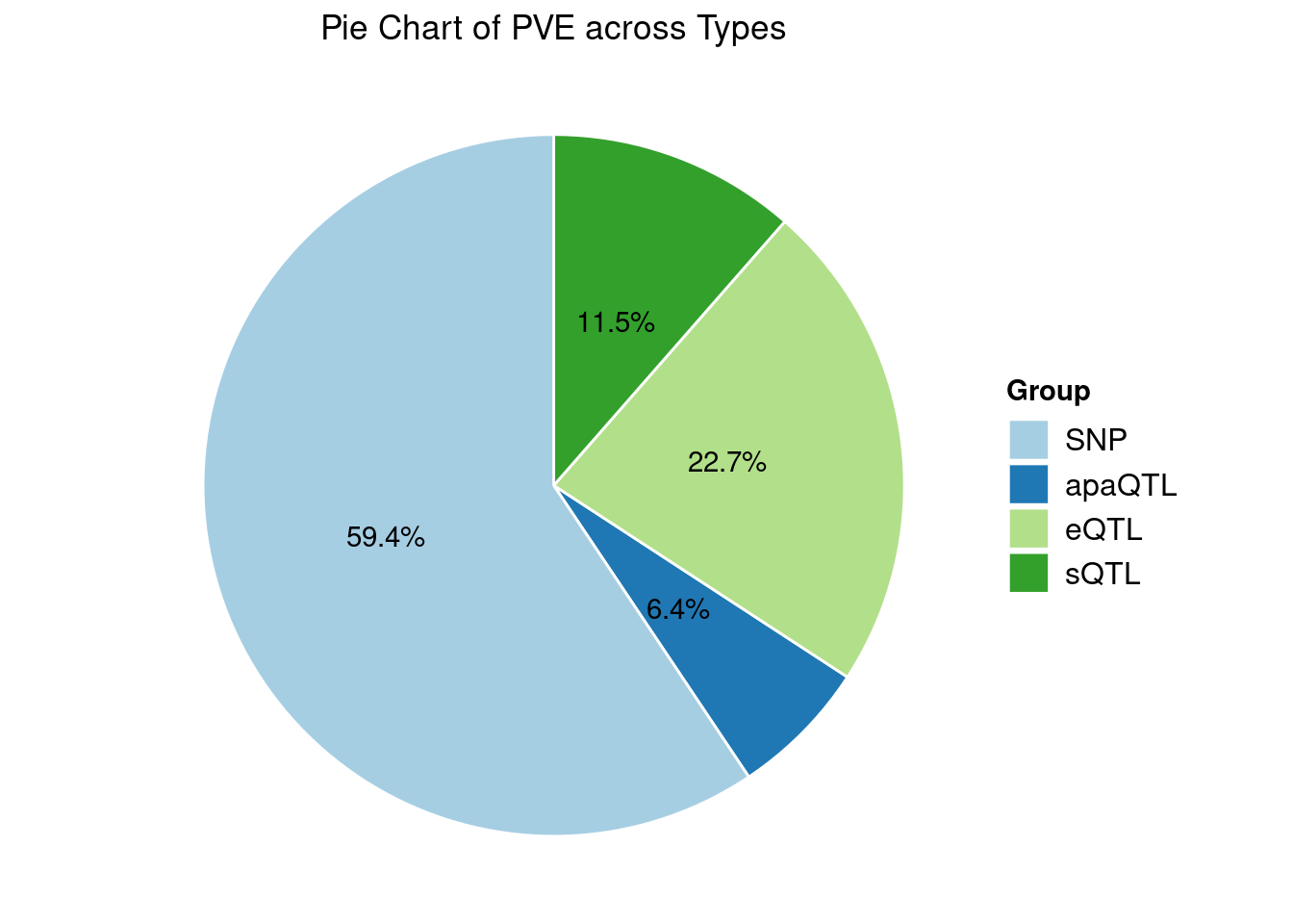
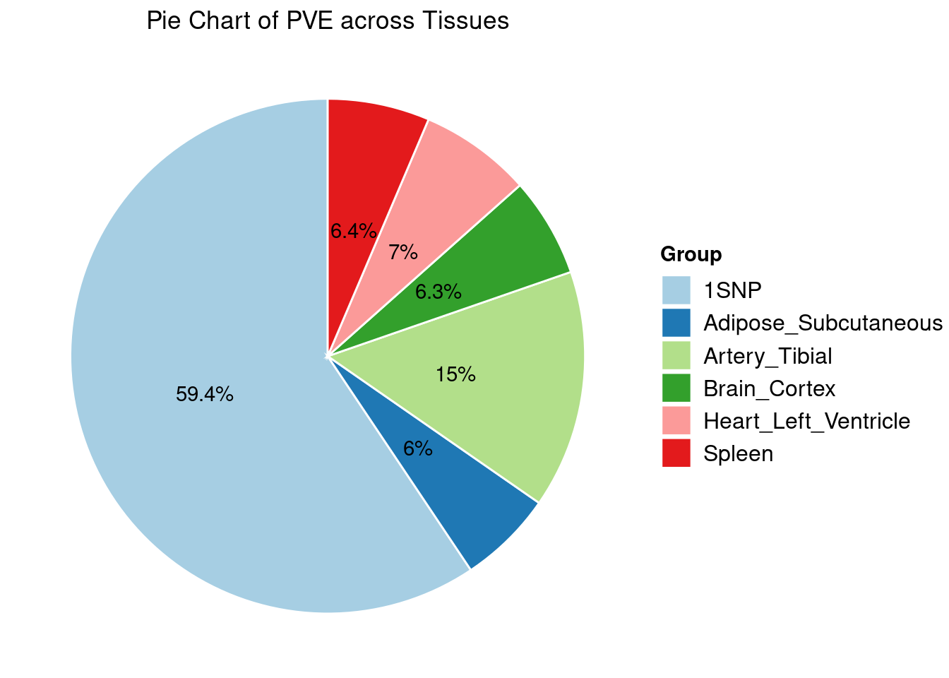
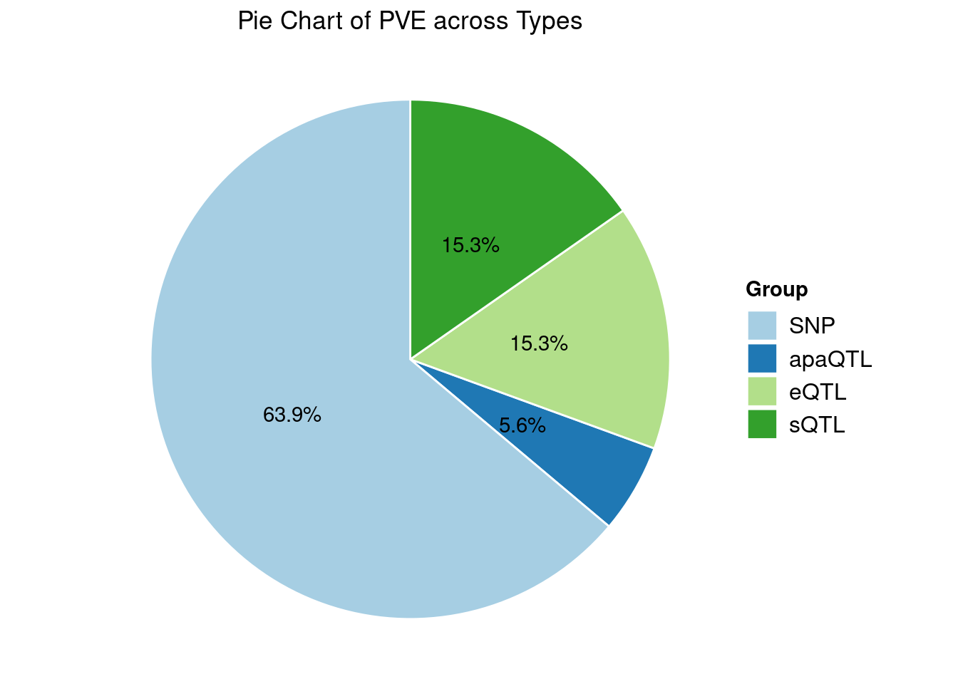
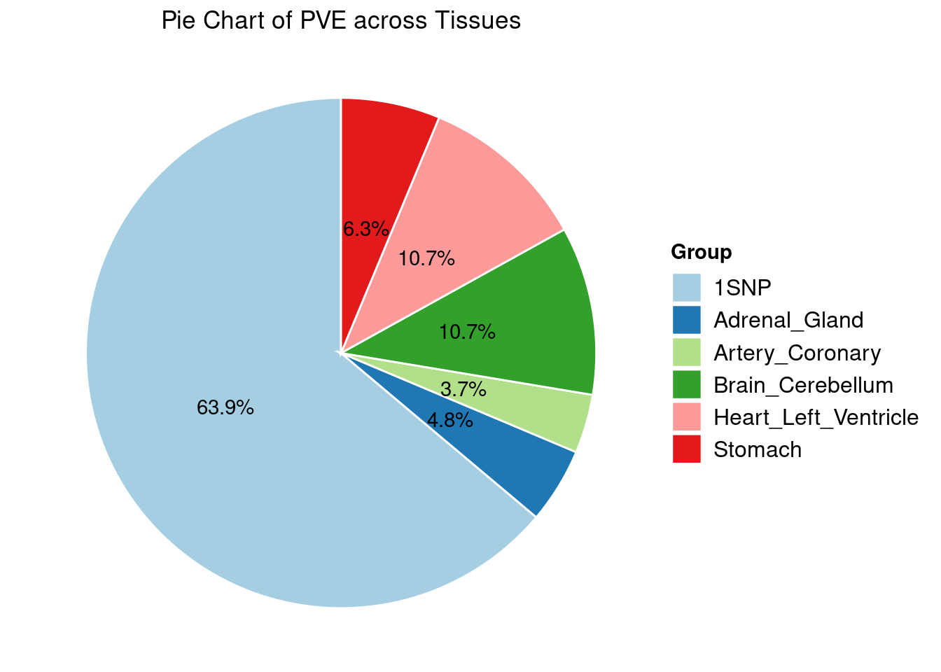
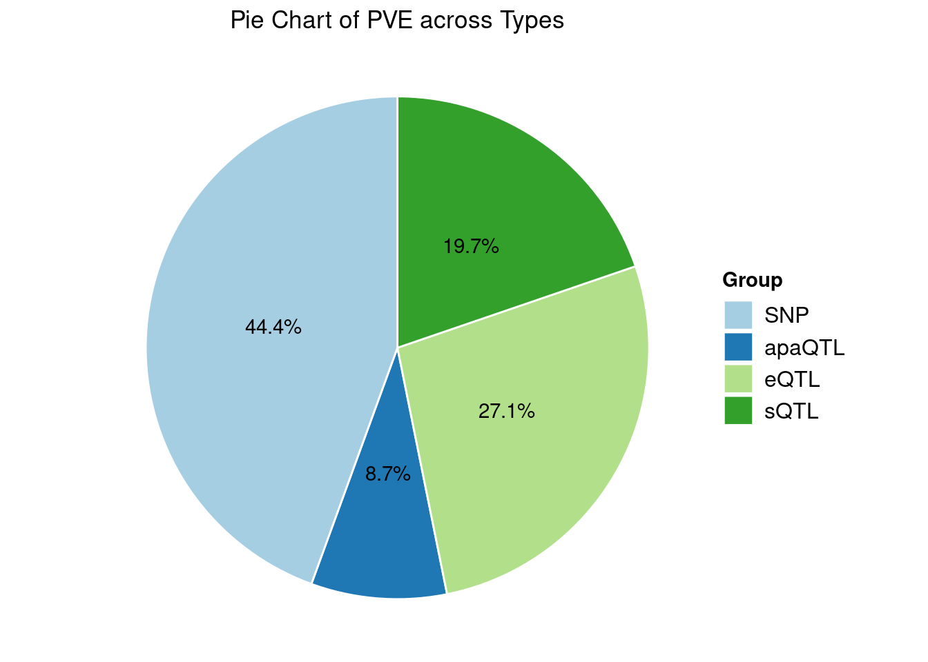
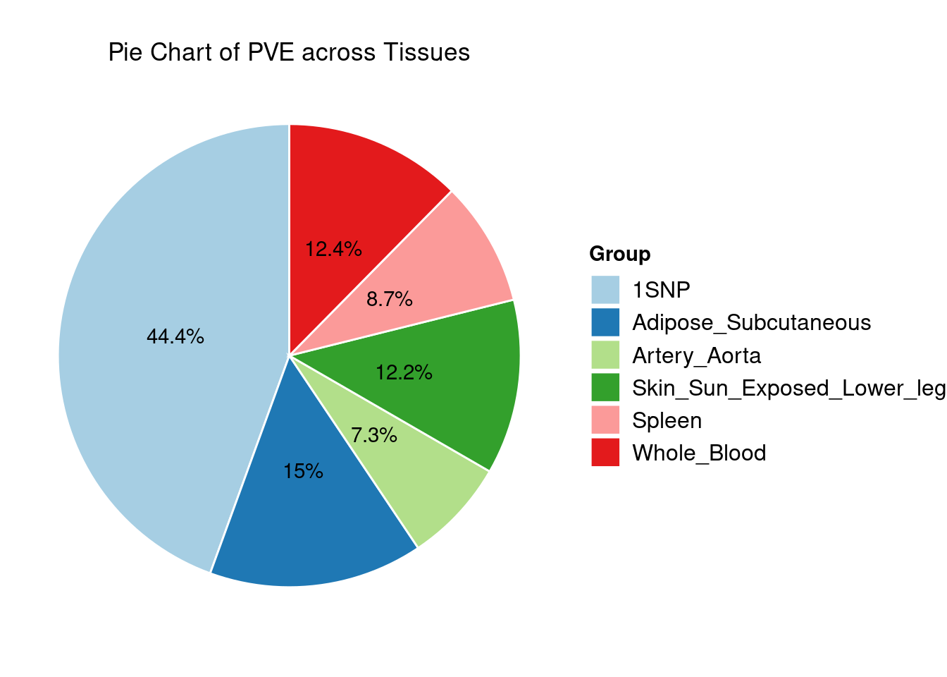
Heritability contribution by contexts: we aggregate the PVE values by omics and tissues, making it easier to understand the distribution of PVE across different genetic contexts.
Combined PIP by omics: we aggregate the Susie PIPs by omics
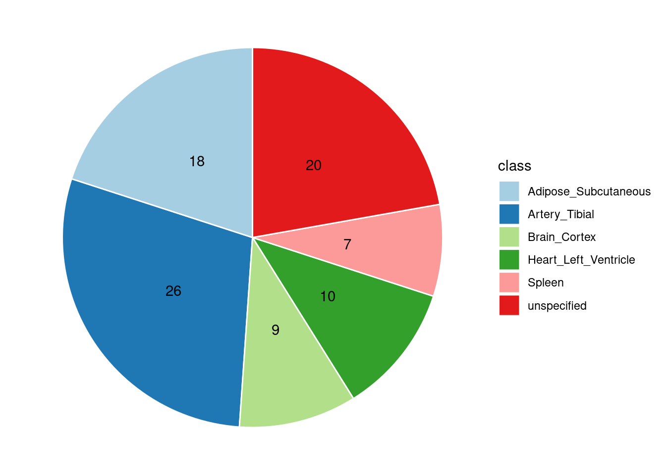
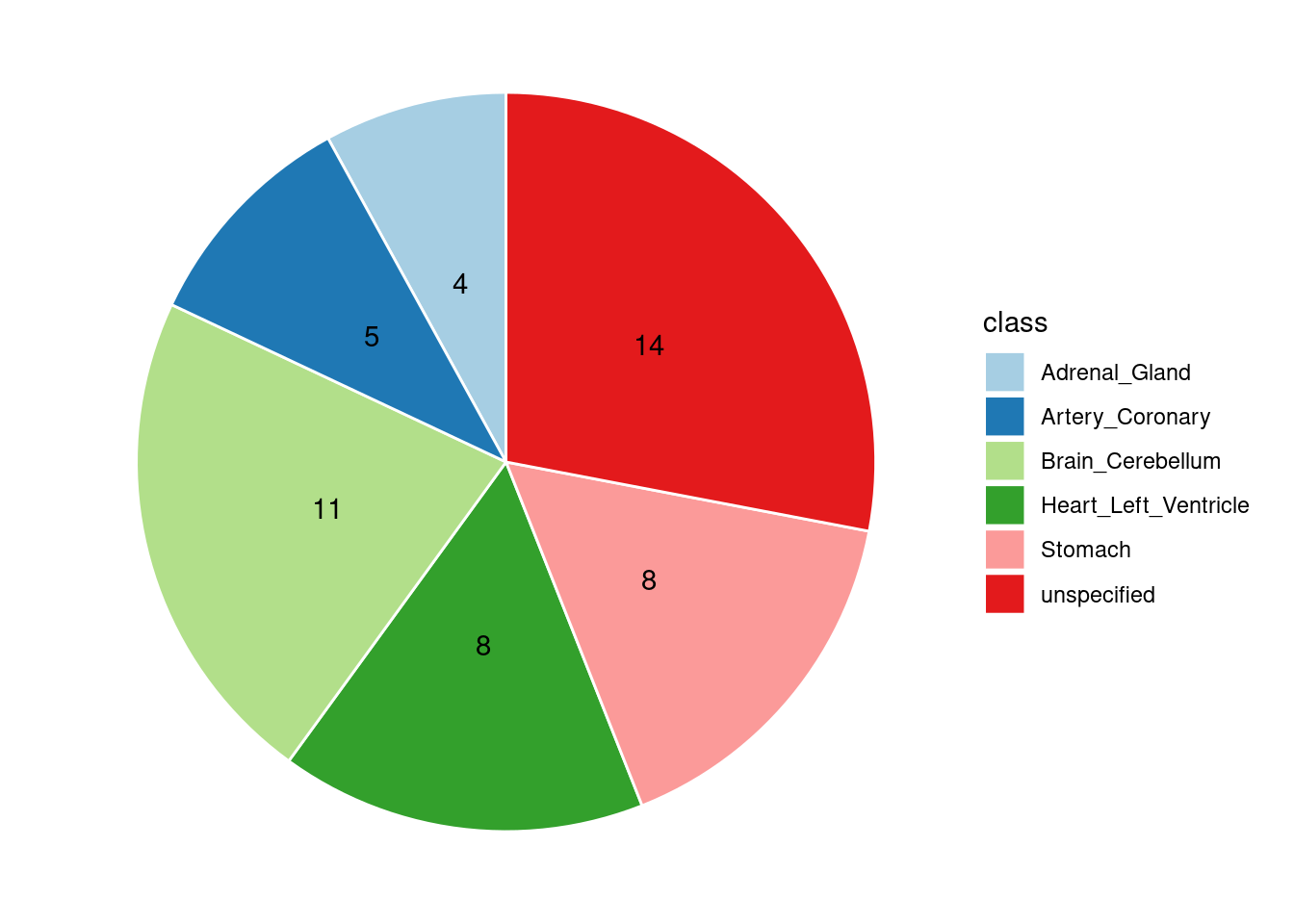
Combined PIP by contexts: we aggregate the Susie PIPs by tissues, making it easier to understand the distribution of PIP across different genetic contexts.
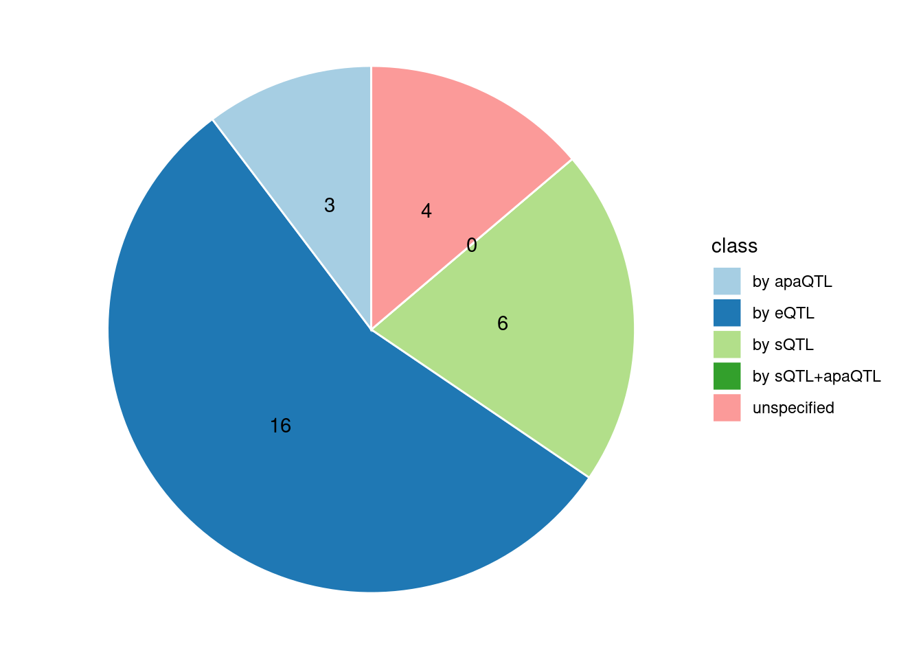
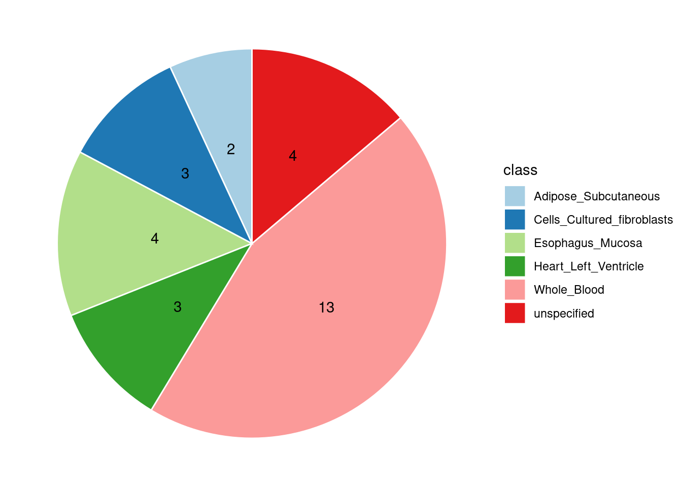
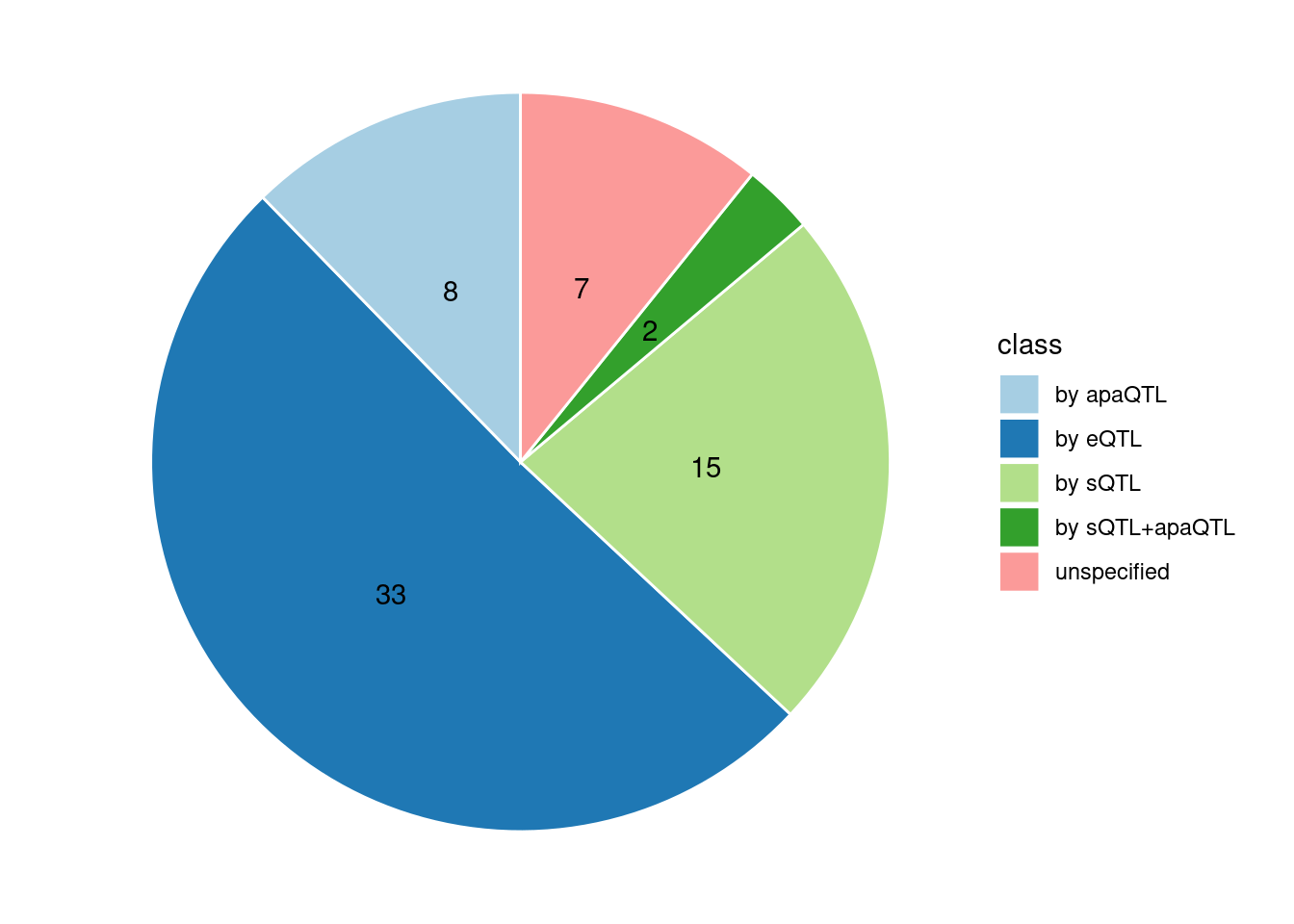
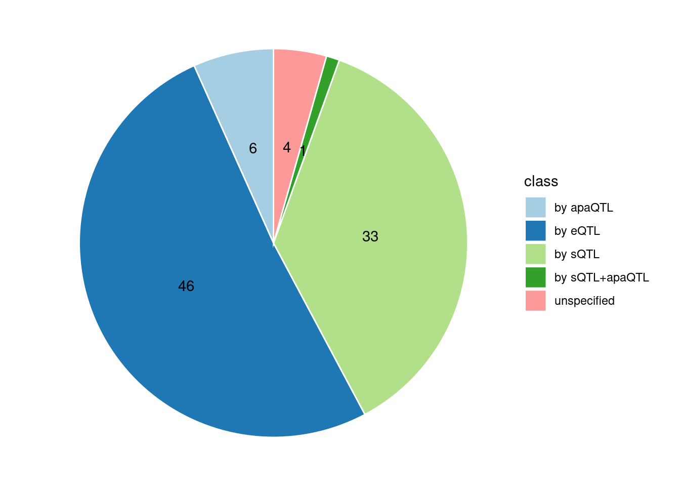
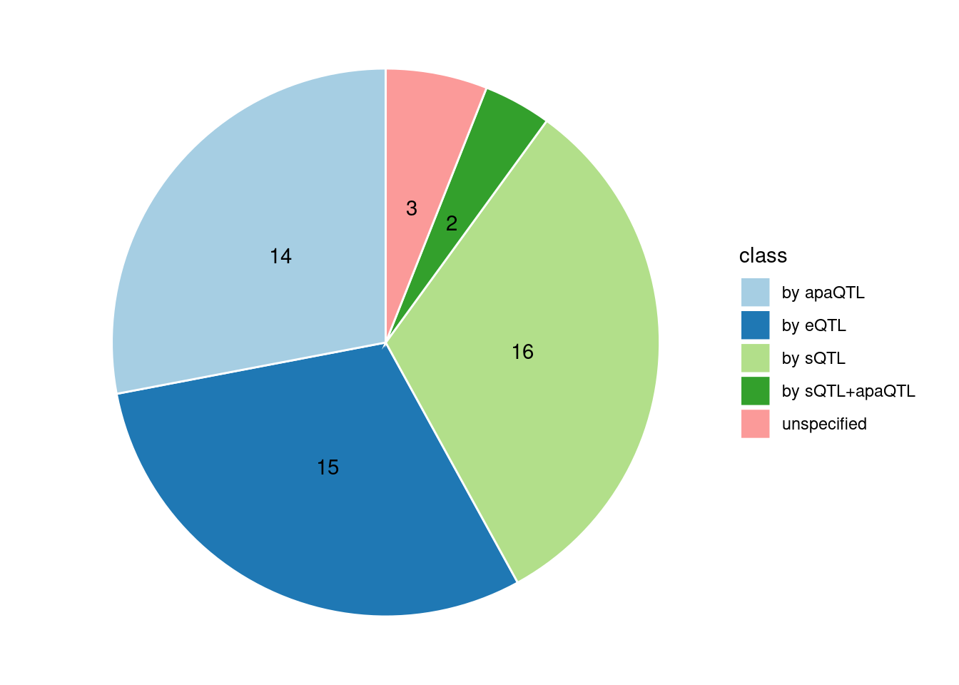
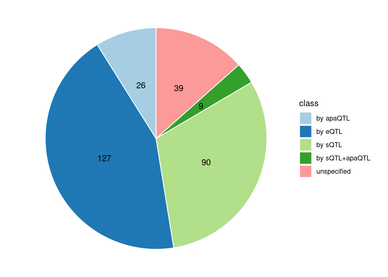
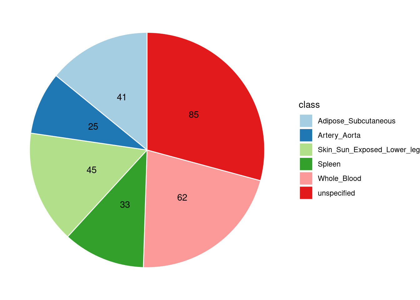
Specific molecular traits of top genes: we creates a pie chart to visualize the proportion of genes classified into different categories based on their PIPs contributed by each genetics contexts. The categories are based on the proportion of each QTL type relative to the combined PIP value:
- by eQTL: Number of genes where the ratio of eQTL to combined PIP is greater than 0.8.
- by sQTL: Number of genes where the ratio of sQTL to combined PIP is greater than 0.8.
- by apaQTL: Number of genes where the ratio of apaQTL to combined PIP is greater than 0.8.
- by sQTL+apaQTL: Number of genes where the combined ratio of apaQTL and sQTL to combined PIP is greater than 0.8, but neither apaQTL nor sQTL individually exceed 0.8.
- unspecified: Number of genes not classified into any of the above categories.
Comparing with single group eQTL results
Please not that the ealier single group eQTL analyses were performed under L=5 but the current analyses were under L=3
We compared number of significant genes, overlapping genes and the changes in PVE for eQTLs across five tissues reported by single eQTL analysi
aFib
TO DO
IBD
Results from multi-group analysis
[1] "Esophagus_Mucosa"           "Adipose_Subcutaneous"
[3] "Whole_Blood"                "Heart_Left_Ventricle"
[5] "Cells_Cultured_fibroblasts"
LDL
Results from multi-group analysis
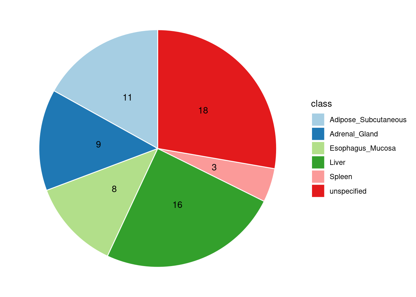
[1] "Esophagus_Mucosa"     "Adipose_Subcutaneous" "Liver"
[4] "Adrenal_Gland" "Spleen" 
SBP
Results from multi-group analysis
[1] "Artery_Tibial"        "Heart_Left_Ventricle" "Spleen"
[4] "Adipose_Subcutaneous" "Brain_Cortex" 
plot for this locus https://uchicago.box.com/s/uca02ksxb4hz67lohjpko35nkjhp5pti
We ran regular SuSiE (uniform prior) in a region, and obtain the number of CS from the results. Then we ran fine-mapping step for this region.
By doing these, we have
estimated_L <- readRDS("/project/xinhe/xsun/multi_group_ctwas/5.multi_group_testing/results_preL/SBP-ukb-a-360/SBP-ukb-a-360.estimated_L.RDS")

sprintf("the pre-estimated L is %s", estimated_L["16:2714828-3951195"])
[1] "the pre-estimated L is 1"load("/project/xinhe/xsun/multi_group_ctwas/5.multi_group_testing/analy_results/NAA60.preL.rdata")
DT::datatable(finemap_res_region_multi,caption = htmltools::tags$caption( style = 'caption-side: topleft; text-align = left; color:black;','Updated PIP (run with pre-estimated L)'),options = list(pageLength = 5) )SCZ
Results from multi-group analysis
[1] "Heart_Left_Ventricle" "Adrenal_Gland"        "Brain_Cerebellum"
[4] "Stomach" "Artery_Coronary" 
WBC
Results from multi-group analysis
[1] "Whole_Blood"                "Skin_Sun_Exposed_Lower_leg"
[3] "Adipose_Subcutaneous"       "Artery_Aorta"
[5] "Spleen" 
sessionInfo()R version 4.2.0 (2022-04-22)
Platform: x86_64-pc-linux-gnu (64-bit)
Running under: CentOS Linux 7 (Core)
Matrix products: default
BLAS/LAPACK: /software/openblas-0.3.13-el7-x86_64/lib/libopenblas_haswellp-r0.3.13.so
locale:
[1] C
attached base packages:
[1] stats graphics grDevices utils datasets methods base
other attached packages:
[1] gridExtra_2.3 RColorBrewer_1.1-3 forcats_0.5.1 stringr_1.5.1
[5] dplyr_1.1.4 purrr_1.0.2 readr_2.1.2 tidyr_1.3.0
[9] tibble_3.2.1 ggplot2_3.5.1 tidyverse_1.3.1 data.table_1.14.2
[13] ctwas_0.2.30
loaded via a namespace (and not attached):
[1] readxl_1.4.0 backports_1.4.1
[3] workflowr_1.7.0 BiocFileCache_2.4.0
[5] plyr_1.8.7 lazyeval_0.2.2
[7] crosstalk_1.2.0 BiocParallel_1.30.3
[9] GenomeInfoDb_1.39.9 LDlinkR_1.2.3
[11] digest_0.6.29 foreach_1.5.2
[13] ensembldb_2.20.2 htmltools_0.5.2
[15] fansi_1.0.3 magrittr_2.0.3
[17] memoise_2.0.1 doParallel_1.0.17
[19] tzdb_0.4.0 Biostrings_2.64.0
[21] modelr_0.1.8 matrixStats_0.62.0
[23] locuszoomr_0.2.1 prettyunits_1.1.1
[25] colorspace_2.0-3 blob_1.2.3
[27] rvest_1.0.2 rappdirs_0.3.3
[29] ggrepel_0.9.1 haven_2.5.0
[31] xfun_0.41 crayon_1.5.1
[33] RCurl_1.98-1.7 jsonlite_1.8.0
[35] zoo_1.8-10 iterators_1.0.14
[37] glue_1.6.2 gtable_0.3.0
[39] zlibbioc_1.42.0 XVector_0.36.0
[41] DelayedArray_0.22.0 BiocGenerics_0.42.0
[43] scales_1.3.0 DBI_1.2.2
[45] Rcpp_1.0.8.3 viridisLite_0.4.0
[47] progress_1.2.2 bit_4.0.4
[49] stats4_4.2.0 DT_0.22
[51] htmlwidgets_1.5.4 httr_1.4.3
[53] ellipsis_0.3.2 pkgconfig_2.0.3
[55] XML_3.99-0.14 farver_2.1.0
[57] sass_0.4.1 dbplyr_2.1.1
[59] utf8_1.2.2 tidyselect_1.2.0
[61] labeling_0.4.2 rlang_1.1.2
[63] later_1.3.0 AnnotationDbi_1.58.0
[65] munsell_0.5.0 pgenlibr_0.3.3
[67] cellranger_1.1.0 tools_4.2.0
[69] cachem_1.0.6 cli_3.6.1
[71] generics_0.1.2 RSQLite_2.3.1
[73] broom_0.8.0 evaluate_0.15
[75] fastmap_1.1.0 yaml_2.3.5
[77] knitr_1.39 bit64_4.0.5
[79] fs_1.5.2 KEGGREST_1.36.3
[81] AnnotationFilter_1.20.0 xml2_1.3.3
[83] biomaRt_2.54.1 compiler_4.2.0
[85] rstudioapi_0.13 plotly_4.10.0
[87] filelock_1.0.2 curl_4.3.2
[89] png_0.1-7 reprex_2.0.1
[91] bslib_0.3.1 stringi_1.7.6
[93] highr_0.9 GenomicFeatures_1.48.3
[95] lattice_0.20-45 ProtGenerics_1.28.0
[97] Matrix_1.5-3 vctrs_0.6.5
[99] pillar_1.9.0 lifecycle_1.0.4
[101] jquerylib_0.1.4 cowplot_1.1.1
[103] bitops_1.0-7 irlba_2.3.5
[105] httpuv_1.6.5 rtracklayer_1.56.0
[107] GenomicRanges_1.48.0 R6_2.5.1
[109] BiocIO_1.6.0 promises_1.2.0.1
[111] IRanges_2.30.0 codetools_0.2-18
[113] assertthat_0.2.1 SummarizedExperiment_1.26.1
[115] rprojroot_2.0.3 rjson_0.2.21
[117] withr_2.5.0 GenomicAlignments_1.32.0
[119] Rsamtools_2.12.0 S4Vectors_0.34.0
[121] GenomeInfoDbData_1.2.8 parallel_4.2.0
[123] hms_1.1.1 grid_4.2.0
[125] gggrid_0.2-0 rmarkdown_2.25
[127] MatrixGenerics_1.8.0 logging_0.10-108
[129] git2r_0.30.1 mixsqp_0.3-43
[131] Biobase_2.56.0 lubridate_1.8.0
[133] restfulr_0.0.14