Multivariate normal: the precision matrix
Matthew Stephens
2016-02-15
Last updated: 2017-02-20
Code version: e778974f2f0b95c6ba67de64e5e5250af4abb052
Pre-requisites
You should be familiar with the multivariate normal distribution and the idea of conditional independence, particularly as illustrated by a Markov Chain.
Overview
This vignette introduces the precision matrix of a multivariate normal. It also illustrates its key property: the zeros of the precision matrix correspond to conditional independencies of the variables.
Definition, and statement of key property
Let \(X\) be multivariate normal with covariance matrix \(\Sigma\).
The precision matrix, \(\Omega\), is simply defined to be the inverse of the covariance matrix: \[\Omega := \Sigma^{-1}\].
The key property of the precision matrix is that its zeros tell you about conditional independence. Specifically: \[\Omega_{ij}=0 \text{ if and only if } X_i \text{ and } X_j \text{ are conditionally independent given all other coordinates of } X.\]
It may help to compare and constrast this with the analogous property of the covariance matrix: \[\Sigma_{ij}=0 \text{ if and only if } X_i \text{ and } X_j \text{ are independent}.\]
That is, whereas zeros of the covariance matrix tell you about independence, zeros of the precision matrix tell you about conditional independence.
Example: A normal markov chain
Consider a Markov chain \(X_1,X_2,X_3,\dots\) where the transitions are given by \(X_{t+1} | X_{t} \sim N(X_{t},1)\). You might think of this Markov chain as corresponding to a type of “random walk”: given the current state, the next state is obtained by adding a random normal with mean 0 and variance 1.
The following code simulates a realization of this Markov chain, starting from an initial state \(X_1 \sim N(0,1)\), and plots it.
set.seed(100)
sim_normal_MC=function(length=1000){
  X = rep(0,length)
  X[1] = rnorm(1)
  for(t in 2:length){
    X[t]= X[t-1] + rnorm(1)
  }
  return(X)
}
plot(sim_normal_MC())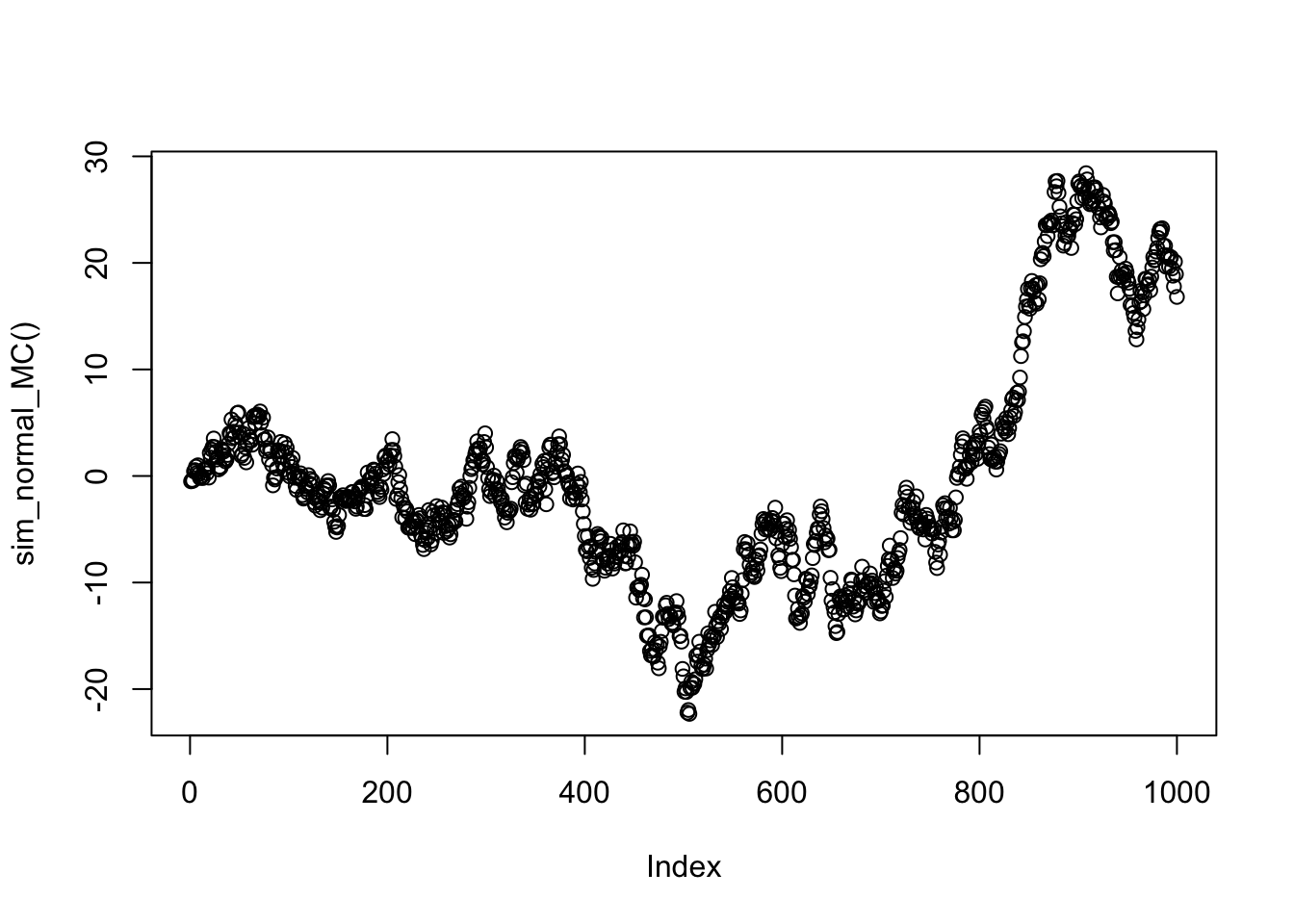
The normal markov chain as a multivariate normal
If you think a little you should be able to see that the above random walk simulation is actually simulating from a 1000-dimensional multivariate normal distribution!
Why?
Well, let’s write each of the \(N(0,1)\) variables we generate using ‘’rnorm’’ in that code as \(Z_1,Z_2,\dots\). Then: \[X_1 = Z_1\] \[X_2 = X_1 + Z_2 = Z_1 + Z_2\] \[X_3 = X_2 + Z_3 = Z_1 + Z_2 + Z_3\] etc.
So we can write \(X = AZ\) where \(A\) is the 1000 by 1000 matrix \[A = \begin{pmatrix} 1 & 0 & 0 & 0 & \dots \\ 1 & 1 & 0 & 0 & \dots \\ 1 & 1 & 1 & 0 & \dots \\ \dots \end{pmatrix}.\]
Let’s take a look at what the covariance matrix Sigma looks like. (We get a good idea from just looking at the top left corner of the matrix what the pattern is)
A = matrix(0,nrow=1000,ncol=1000)
for(i in 1:1000){
    A[i,]=c(rep(1,i),rep(0,1000-i))
}
Sigma = A %*% t(A)
Sigma[1:10,1:10]
[,1] [,2] [,3] [,4] [,5] [,6] [,7] [,8] [,9] [,10]
[1,] 1 1 1 1 1 1 1 1 1 1
[2,] 1 2 2 2 2 2 2 2 2 2
[3,] 1 2 3 3 3 3 3 3 3 3
[4,] 1 2 3 4 4 4 4 4 4 4
[5,] 1 2 3 4 5 5 5 5 5 5
[6,] 1 2 3 4 5 6 6 6 6 6
[7,] 1 2 3 4 5 6 7 7 7 7
[8,] 1 2 3 4 5 6 7 8 8 8
[9,] 1 2 3 4 5 6 7 8 9 9
[10,] 1 2 3 4 5 6 7 8 9 10Now let us examine the precision matrix, \(\Omega\), which recall is the inverse of \(\Sigma\). Again we just show the top left corner of the precision matrix here.
Omega = chol2inv(chol(Sigma))
Omega[1:10,1:10]
[,1] [,2] [,3] [,4] [,5] [,6] [,7] [,8] [,9] [,10]
[1,] 2 -1 0 0 0 0 0 0 0 0
[2,] -1 2 -1 0 0 0 0 0 0 0
[3,] 0 -1 2 -1 0 0 0 0 0 0
[4,] 0 0 -1 2 -1 0 0 0 0 0
[5,] 0 0 0 -1 2 -1 0 0 0 0
[6,] 0 0 0 0 -1 2 -1 0 0 0
[7,] 0 0 0 0 0 -1 2 -1 0 0
[8,] 0 0 0 0 0 0 -1 2 -1 0
[9,] 0 0 0 0 0 0 0 -1 2 -1
[10,] 0 0 0 0 0 0 0 0 -1 2Notice all the 0s in the precision matrix. This is because of the conditional independencies that occur in a Markov chain. In a Markov chain (any Markov chain) the conditional distribution of \(X_t\) given the other \(X_s\) (\(s \neq t\)) depends only on its neighbors \(X_{t-1}\) and \(X_{t+1}\). That is, \(X_{t}\) is conditionally independent of all other \(X_s\) given \(X_{t-1}\) and \(X_{t+1}\). This is exactly what we are seeing in the precision matrix above: the non-zero elements of the \(t\)th row are at coordinates \(t-1,t\) and \(t+1\).
Session information
sessionInfo()R version 3.3.2 (2016-10-31)
Platform: x86_64-apple-darwin13.4.0 (64-bit)
Running under: OS X El Capitan 10.11.6
locale:
[1] en_US.UTF-8/en_US.UTF-8/en_US.UTF-8/C/en_US.UTF-8/en_US.UTF-8
attached base packages:
[1] stats graphics grDevices utils datasets methods base
other attached packages:
[1] workflowr_0.3.0 rmarkdown_1.3 ggplot2_2.2.1 dplyr_0.5.0
[5] magrittr_1.5 shiny_1.0.0 mixfdr_1.0 ashr_2.1.2
[9] dscr_0.1.1 horseshoe_0.1.0
loaded via a namespace (and not attached):
[1] Rcpp_0.12.9 git2r_0.18.0 plyr_1.8.4
[4] iterators_1.0.8 tools_3.3.2 digest_0.6.12
[7] memoise_1.0.0 tibble_1.2 jsonlite_1.2
[10] evaluate_0.10 gtable_0.2.0 lattice_0.20-34
[13] Matrix_1.2-7.1 foreach_1.4.3 DBI_0.5-1
[16] rstudioapi_0.6 curl_2.2 yaml_2.1.14
[19] parallel_3.3.2 httr_1.2.1 withr_1.0.2
[22] stringr_1.1.0 knitr_1.15.1 devtools_1.12.0
[25] REBayes_0.73 rprojroot_1.2 grid_3.3.2
[28] R6_2.2.0 EbayesThresh_1.3.2 reshape2_1.4.2
[31] whisker_0.3-2 backports_1.0.5 scales_0.4.1
[34] codetools_0.2-15 htmltools_0.3.5 MASS_7.3-45
[37] assertthat_0.1 mime_0.5 colorspace_1.2-7
[40] xtable_1.8-2 httpuv_1.3.3 labeling_0.3
[43] stringi_1.1.2 Rmosek_7.1.2 lazyeval_0.2.0
[46] munsell_0.4.3 doParallel_1.0.10 pscl_1.4.9
[49] truncnorm_1.0-7 SQUAREM_2016.8-2 This site was created with R Markdown