Introduction to bivariate normal distribution
Matthew Stephens
2022-03-01
Last updated: 2022-03-01
Checks: 7 0
Knit directory: fiveMinuteStats/analysis/
This reproducible R Markdown analysis was created with workflowr (version 1.7.0). The Checks tab describes the reproducibility checks that were applied when the results were created. The Past versions tab lists the development history.
Great! Since the R Markdown file has been committed to the Git repository, you know the exact version of the code that produced these results.
Great job! The global environment was empty. Objects defined in the global environment can affect the analysis in your R Markdown file in unknown ways. For reproduciblity it’s best to always run the code in an empty environment.
The command set.seed(12345) was run prior to running the code in the R Markdown file. Setting a seed ensures that any results that rely on randomness, e.g. subsampling or permutations, are reproducible.
Great job! Recording the operating system, R version, and package versions is critical for reproducibility.
Nice! There were no cached chunks for this analysis, so you can be confident that you successfully produced the results during this run.
Great job! Using relative paths to the files within your workflowr project makes it easier to run your code on other machines.
Great! You are using Git for version control. Tracking code development and connecting the code version to the results is critical for reproducibility.
The results in this page were generated with repository version ea5b4f3. See the Past versions tab to see a history of the changes made to the R Markdown and HTML files.
Note that you need to be careful to ensure that all relevant files for the analysis have been committed to Git prior to generating the results (you can use wflow_publish or wflow_git_commit). workflowr only checks the R Markdown file, but you know if there are other scripts or data files that it depends on. Below is the status of the Git repository when the results were generated:
Ignored files:
    Ignored:    .Rhistory
    Ignored:    .Rproj.user/
    Ignored:    analysis/.Rhistory
    Ignored:    analysis/bernoulli_poisson_process_cache/

Untracked files:
    Untracked:  _workflowr.yml
    Untracked:  analysis/CI.Rmd
    Untracked:  analysis/gibbs_structure.Rmd
    Untracked:  analysis/libs/
    Untracked:  analysis/results.Rmd
    Untracked:  analysis/shiny/tester/

Unstaged changes:
    Modified:   analysis/LR_and_BF.Rmd
    Modified:   analysis/MH-examples1.Rmd
    Modified:   analysis/MH_intro.Rmd
    Deleted:    analysis/r_simplemix_extended.Rmd
Note that any generated files, e.g. HTML, png, CSS, etc., are not included in this status report because it is ok for generated content to have uncommitted changes.
These are the previous versions of the repository in which changes were made to the R Markdown (analysis/mvnorm_00.Rmd) and HTML (docs/mvnorm_00.html) files. If you’ve configured a remote Git repository (see ?wflow_git_remote), click on the hyperlinks in the table below to view the files as they were in that past version.
| File | Version | Author | Date | Message |
|---|---|---|---|---|
| Rmd | ea5b4f3 | Matthew Stephens | 2022-03-01 | workflowr::wflow_publish(“mvnorm_00.Rmd”) |
| html | 77d271e | Matthew Stephens | 2022-03-01 | Build site. |
| Rmd | a9ceaa1 | Matthew Stephens | 2022-03-01 | workflowr::wflow_publish(“mvnorm_00.Rmd”) |
Pre-requisites
You need to have basic familiarity with univariate normal distribution, and understand the basic property that linear combinations of normals are also normal.
Motivating example
Suppose that \(Z_1,Z_2\) are independent standard normal \(N(0,1)\) and define \(X_1=Z_1+0.1 Z_2\) and \(X_2=Z_1-0.1 Z_2\). What is the joint distribution of \(X_1,X_2\)?
We know from the basic property that \(X_1\) will be univariate normal, and that \(X_2\) will be univariate normal. However, they will not necessarily be independent because \(Z_1\) and \(Z_2\) were used to compute both. Indeed, you can see that \(X_1\) and \(X_2\) might both be expected to be close to \(Z_1\) (because the 0.1 multiplier on \(Z_2\) is “relatively small”). So when \(X_1\) is big we should expect \(X_2\) will likely be big, and when \(X_1\) is small we should expect \(X_2\) will likely small.
The following code illustrates this: the histograms illustrate both \(X_1\) and \(X_2\) are normal, and the scatterplot of \(X_1\) and \(X_2\) shows they are correlated (and the sample correlation is approximately 0.98).
Z1 = rnorm(1000)
Z2 = rnorm(1000)

X1 = Z1+0.1*Z2
X2 = Z1-0.1*Z2

hist(X1)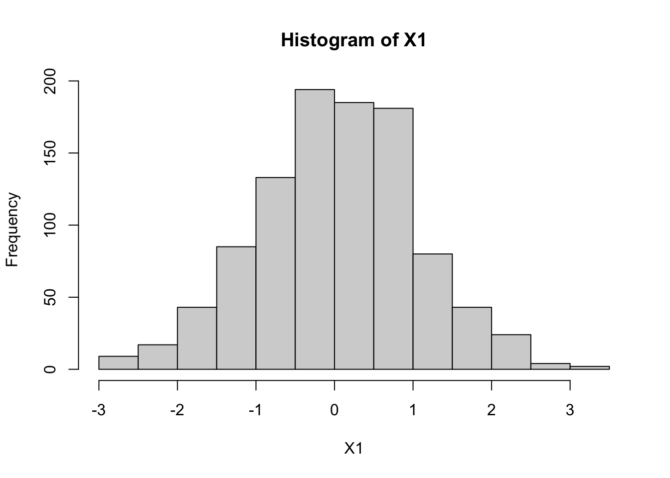
| Version | Author | Date |
|---|---|---|
| 77d271e | Matthew Stephens | 2022-03-01 |
hist(X2)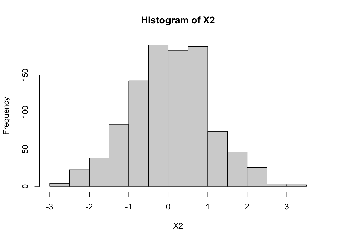
| Version | Author | Date |
|---|---|---|
| 77d271e | Matthew Stephens | 2022-03-01 |
plot(X1,X2, main="scatterplot of (X1,X2)", ylim=c(-4,4), asp=1) #asp=1 sets the scales of X1 and X2 the same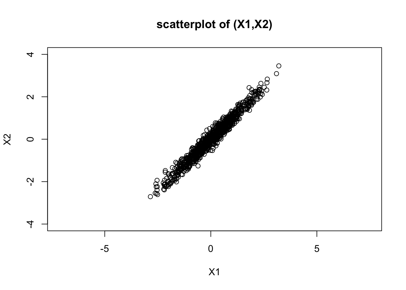
| Version | Author | Date |
|---|---|---|
| 77d271e | Matthew Stephens | 2022-03-01 |
cor(X1,X2)[1] 0.9798486The bivariate normal distribution
In fact the answer to the question “what is the joint distribution of \(X_1,X_2\)” is they have a “bivariate normal distribution”. Thus the scatterplot shown above shows a scatterplot of 1000 samples from a bivariate normal distribution. The prefix “bi” means 2, referring to the fact that here we are looking at 2 variables, \(X_1\) and \(X_2\). The ideas here can be extended to more variables, and the resulting distribution is called the “multivariate normal”. The bivariate normal is a special case of the multivariate normal.
Mean and Covariance Matrix
The bivariate normal distribution has 5 parameters: two means (for \(X_1\) and \(X_2\)), two variances (for \(X_1\) and \(X_2\)) and the covariance between \(X_1\) and \(X_2\). It is usual to write the mean parameter as a vector \(\mu\) and the variance and covariance parameters as a 2x2 symmetric matrix \(\Sigma\), where the diagonal elements of \(\Sigma\) contain the variances and the off-diagonal elements contain the covariance. \(\Sigma\) is called the “covariance matrix” (or sometimes the “variance-covariance matrix”).
General Construction
Suppose \(Z_1,Z_2\) are independent random variables each with a standard normal distribution \(N(0,1)\). Let \(Z\) denote the vector \((Z_1,Z_2)\), let \(A\) be any \(2 \times 2\) matrix, and \(\mu\) be any \(r\)-vector. Then the vector \(X = AZ+\mu\) has a bivariate normal distribution with mean \(\mu\) and variance-covariance matrix \(\Sigma=AA'\). (Here \(A'\) means the transpose of the matrix \(A\).) We write \(X \sim N_2(\mu,\Sigma)\).
Example
We can redo the example above in vector and matrix notation, with \(\mu=(0,0)\) and \(A=(1,0.1),(1,-0.1)\). Here for clarity we just simulate a single sample instead of 1000:
mu = c(0,0)
A = rbind(c(1,0.1),c(1,-0.1))
A
[,1] [,2]
[1,] 1 0.1
[2,] 1 -0.1z = rnorm(2)
x = mu + A %*% z
x [,1]
[1,] -0.5002188
[2,] -0.7154634It should be clear from the above that in our example the mean is \(\mu=(0,0)\). What is the covariance matrix \(\Sigma\)? We can compute it from the formula \(\Sigma = AA'\):
Sigma = A %*% t(A)
Sigma
[,1] [,2]
[1,] 1.01 0.99
[2,] 0.99 1.01
sessionInfo()R version 4.1.0 Patched (2021-07-20 r80657)
Platform: aarch64-apple-darwin20 (64-bit)
Running under: macOS Monterey 12.2
Matrix products: default
BLAS: /Library/Frameworks/R.framework/Versions/4.1-arm64/Resources/lib/libRblas.0.dylib
LAPACK: /Library/Frameworks/R.framework/Versions/4.1-arm64/Resources/lib/libRlapack.dylib
locale:
[1] en_US.UTF-8/en_US.UTF-8/en_US.UTF-8/C/en_US.UTF-8/en_US.UTF-8
attached base packages:
[1] stats graphics grDevices utils datasets methods base
loaded via a namespace (and not attached):
[1] Rcpp_1.0.7 whisker_0.4 knitr_1.36 magrittr_2.0.2
[5] workflowr_1.7.0 R6_2.5.1 rlang_0.4.12 fastmap_1.1.0
[9] fansi_0.5.0 highr_0.9 stringr_1.4.0 tools_4.1.0
[13] xfun_0.28 utf8_1.2.2 git2r_0.29.0 jquerylib_0.1.4
[17] htmltools_0.5.2 ellipsis_0.3.2 rprojroot_2.0.2 yaml_2.2.1
[21] digest_0.6.28 tibble_3.1.6 lifecycle_1.0.1 crayon_1.4.2
[25] later_1.3.0 vctrs_0.3.8 fs_1.5.0 promises_1.2.0.1
[29] glue_1.5.0 evaluate_0.14 rmarkdown_2.11 stringi_1.7.5
[33] compiler_4.1.0 pillar_1.6.4 httpuv_1.6.3 pkgconfig_2.0.3 This site was created with R Markdown