Simulating Discrete Markov Chains: An Introduction
Matt Bonakdarpour
2016-01-21
Last updated: 2019-03-31
Checks: 6 0
Knit directory: fiveMinuteStats/analysis/
This reproducible R Markdown analysis was created with workflowr (version 1.2.0). The Report tab describes the reproducibility checks that were applied when the results were created. The Past versions tab lists the development history.
Great! Since the R Markdown file has been committed to the Git repository, you know the exact version of the code that produced these results.
Great job! The global environment was empty. Objects defined in the global environment can affect the analysis in your R Markdown file in unknown ways. For reproduciblity it’s best to always run the code in an empty environment.
The command set.seed(12345) was run prior to running the code in the R Markdown file. Setting a seed ensures that any results that rely on randomness, e.g. subsampling or permutations, are reproducible.
Great job! Recording the operating system, R version, and package versions is critical for reproducibility.
Nice! There were no cached chunks for this analysis, so you can be confident that you successfully produced the results during this run.
Great! You are using Git for version control. Tracking code development and connecting the code version to the results is critical for reproducibility. The version displayed above was the version of the Git repository at the time these results were generated.
Note that you need to be careful to ensure that all relevant files for the analysis have been committed to Git prior to generating the results (you can use wflow_publish or wflow_git_commit). workflowr only checks the R Markdown file, but you know if there are other scripts or data files that it depends on. Below is the status of the Git repository when the results were generated:
Ignored files:
    Ignored:    .Rhistory
    Ignored:    .Rproj.user/
    Ignored:    analysis/.Rhistory
    Ignored:    analysis/bernoulli_poisson_process_cache/

Untracked files:
    Untracked:  _workflowr.yml
    Untracked:  analysis/CI.Rmd
    Untracked:  analysis/gibbs_structure.Rmd
    Untracked:  analysis/libs/
    Untracked:  analysis/results.Rmd
    Untracked:  analysis/shiny/tester/
    Untracked:  docs/MH_intro_files/
    Untracked:  docs/citations.bib
    Untracked:  docs/figure/MH_intro.Rmd/
    Untracked:  docs/figure/hmm.Rmd/
    Untracked:  docs/hmm_files/
    Untracked:  docs/libs/
    Untracked:  docs/shiny/tester/
Note that any generated files, e.g. HTML, png, CSS, etc., are not included in this status report because it is ok for generated content to have uncommitted changes.
These are the previous versions of the R Markdown and HTML files. If you’ve configured a remote Git repository (see ?wflow_git_remote), click on the hyperlinks in the table below to view them.
| File | Version | Author | Date | Message |
|---|---|---|---|---|
| html | 34bcc51 | John Blischak | 2017-03-06 | Build site. |
| Rmd | 5fbc8b5 | John Blischak | 2017-03-06 | Update workflowr project with wflow_update (version 0.4.0). |
| Rmd | 391ba3c | John Blischak | 2017-03-06 | Remove front and end matter of non-standard templates. |
| html | fb0f6e3 | stephens999 | 2017-03-03 | Merge pull request #33 from mdavy86/f/review |
| html | c3b365a | John Blischak | 2017-01-02 | Build site. |
| Rmd | 67a8575 | John Blischak | 2017-01-02 | Use external chunk to set knitr chunk options. |
| Rmd | 5ec12c7 | John Blischak | 2017-01-02 | Use session-info chunk. |
| Rmd | dfaabc4 | mbonakda | 2016-02-02 | spin off inverse transform sampling into its own note |
| Rmd | f209a9a | mbonakda | 2016-01-30 | fix up typos |
| Rmd | ad8b7b5 | mbonakda | 2016-01-30 | update names |
| Rmd | 0f93e3c | mbonakda | 2016-01-30 | split simulating discrete markov chains into three separate notes |
Pre-requisites
This document assumes basic familiarity with Markov chains.
Illustrative Example
In this note, we will describe a simple algorithm for simulating Markov chains. We first settle on notation and describe the algorithm in words.
Let \(P_{ij}\) denote the one-step transition probability. That is, \[ P_{ij} = P(X_{t+1} = j | X_{t} = i)\]
In what follows, we will assume that the transition probabilities do not depend on time \(t\). These are called time homogenous Markov chains.
The general idea of simulating discrete Markov chains can be illustrated through a simple example with 2 states. Assume our state space is \(\{1,2\}\) and the transition matrix is:
\[P = \begin{bmatrix} 0.7 & 0.3 \\ 0.4 & 0.6 \end{bmatrix}\]
We denote the \((i,j)\)-th entry of the matrix \(P\) as \(P_{ij}\).
Now assume that our Markov chain starts in state 1 so that \(X_0 = 1\). Since we are starting in state 1, our transition probabilities are defined by the first row of \(P\). Our chain can either remain in state \(1\) with probability \(P_{11}\) or transition to state \(2\) with probability \(P_{12}\). Therefore, to simulate \(X_1\), we must generate a random variable according to the probabilities \(P_{11}= P(X_1 = 1 | X_0 = 1) = 0.7\) and \(P_{12} = P(X_1 = 2 | X_0 = 0) = 0.3\).
In general, we can generate any discrete random variable according to a set of probabilities \(p = \{p_1, \ldots, p_K\}\) with Inverse Transform Sampling. Also note that this is equivalent to taking a single draw from a multinomial distribution with probability vector \(p\) – we use this method in the algorithm below.
General Algorithm
Here we present a general algorithm for simulating a discrete Markov chain assuming we have \(S\) possible states.
- Obtain the \(S\times S\) probability transition matrix \(P\)
- Set \(t = 0\)
- Pick an initial state \(X_t=i\).
- For t = 1…T:
- Obtain the row of \(P\) corresponding to the current state \(X_t\).
- Generate \(X_{t+1}\) from a multinomial distribution with probability vector equal to the row we obtained above.
We implement this in the following function, initializing the first state to \(1\):
# simulate discrete Markov chains according to transition matrix P
run.mc.sim <- function( P, num.iters = 50 ) {

  # number of possible states
  num.states <- nrow(P)

  # stores the states X_t through time
  states     <- numeric(num.iters)

  # initialize variable for first state
  states[1]    <- 1

  for(t in 2:num.iters) {

    # probability vector to simulate next state X_{t+1}
    p  <- P[states[t-1], ]

    ## draw from multinomial and determine state
    states[t] <-  which(rmultinom(1, 1, p) == 1)
  }
  return(states)
}
Simulation 1: 3x3 example
Assume our probability transition matrix is: \[P = \begin{bmatrix} 0.7 & 0.2 & 0.1 \\ 0.4 & 0.6 & 0 \\ 0 & 1 & 0 \end{bmatrix}\]
We initialize this matrix in R below:
# setup transition matrix
P <- t(matrix(c( 0.7, 0.2, 0.1,
                 0.4, 0.6,   0,
                   0,   1,   0  ), nrow=3, ncol=3))
Now we will use the function we wrote in the previous section to run several chains and plot the results:
num.chains     <- 5
num.iterations <- 50

# each column stores the sequence of states for a single chains
chain.states  <- matrix(NA, ncol=num.chains, nrow=num.iterations)

# simulate chains
for(c in seq_len(num.chains)){
  chain.states[,c] <- run.mc.sim(P)
}
Our function returns a vector that contains the states of our simulated chain through time. Recall that our state space is \(\{1,2,3\}\). Below, we visualize how these chains evolve through time:
matplot(chain.states, type='l', lty=1, col=1:5, ylim=c(0,4), ylab='state', xlab='time')
abline(h=1, lty=3)
abline(h=3, lty=3)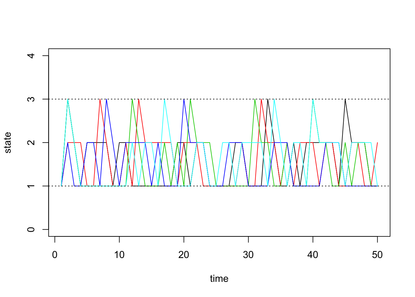
| Version | Author | Date |
|---|---|---|
| c3b365a | John Blischak | 2017-01-02 |
Simulation 2: 8x8 example
Next we will do a larger experiment with the size of our state space equal to 8. Assume our probability transition matrix is: \[P = \begin{bmatrix} 0.33 & 0.66 & 0 & 0 & 0 & 0 & 0 & 0 \\ 0.33 & 0.33 & 0.33 & 0 & 0 & 0 & 0 & 0 \\ 0 & 0.33 & 0.33 & 0.33 & 0 & 0 & 0 & 0 \\ 0 & 0 & 0.33 & 0.33 & 0.33 & 0 & 0 & 0 \\ 0 & 0 & 0 & 0.33 & 0.33 & 0.33 & 0 & 0 \\ 0 & 0 & 0 & 0 & 0.33 & 0.33 & 0.33 & 0 \\ 0 & 0 & 0 & 0 & 0 & 0.33 & 0.33 & 0.33 \\ 0 & 0 & 0 & 0 & 0 & 0 & 0.66 & 0.33 \\ \end{bmatrix}\]
We first initialize our transition matrix in R:
P <- t(matrix(c( 1/3, 2/3,   0,   0,  0,   0,   0,   0,
                 1/3, 1/3, 1/3,   0,  0,   0,   0,   0,
                   0, 1/3, 1/3, 1/3,  0,   0,   0,   0,
                   0,   0, 1/3, 1/3, 1/3,  0,   0,   0,
                   0,   0,   0, 1/3, 1/3, 1/3,  0,   0,
                   0,   0,   0,   0, 1/3, 1/3, 1/3,  0,
                   0,   0,   0,   0,   0, 1/3, 1/3, 1/3,
                   0,   0,   0,   0,   0,   0, 2/3, 1/3), nrow=8, ncol=8))
After briefly studying this matrix, we can see that for states 2 through 7, this transition matrix forces the chain to either stay in the current state or move one state up or down, all with equal probability. For the edge cases, states 1 and 8, the chain can either stay or reflect towards the middle states.
Now we run our simulations with the transition matrix above:
num.chains     <- 5
num.iterations <- 50
chain.states <- matrix(NA, ncol=num.chains, nrow=num.iterations)
for(c in seq_len(num.chains)){
  chain.states[,c] <- run.mc.sim(P)
}
And finally we plot the chains through time below:
matplot(chain.states, type='l', lty=1, col=1:5, ylim=c(0,9), ylab='state', xlab='time')
abline(h=1, lty=3)
abline(h=8, lty=3)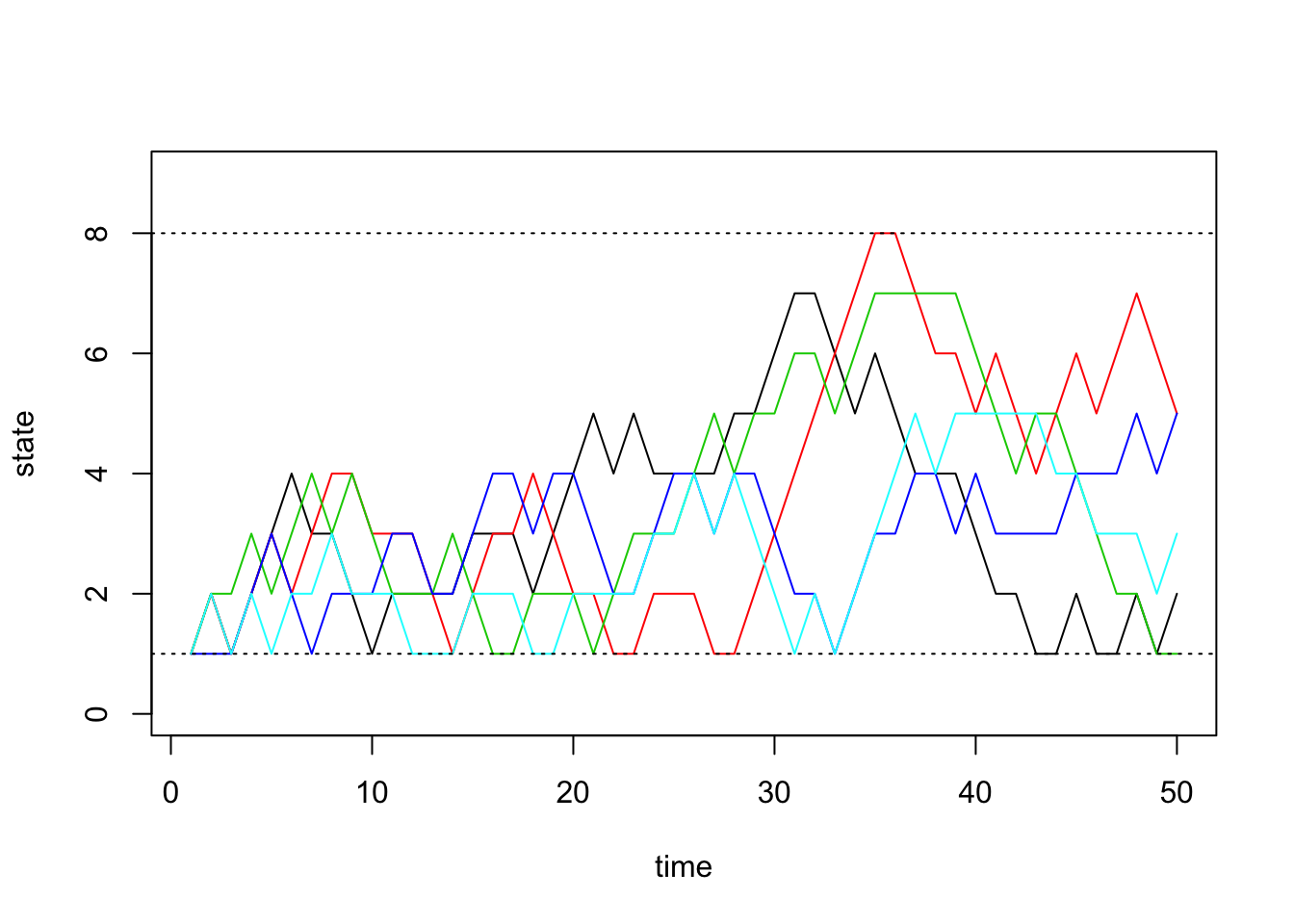
| Version | Author | Date |
|---|---|---|
| c3b365a | John Blischak | 2017-01-02 |
sessionInfo()R version 3.5.2 (2018-12-20)
Platform: x86_64-apple-darwin15.6.0 (64-bit)
Running under: macOS Mojave 10.14.1
Matrix products: default
BLAS: /Library/Frameworks/R.framework/Versions/3.5/Resources/lib/libRblas.0.dylib
LAPACK: /Library/Frameworks/R.framework/Versions/3.5/Resources/lib/libRlapack.dylib
locale:
[1] en_US.UTF-8/en_US.UTF-8/en_US.UTF-8/C/en_US.UTF-8/en_US.UTF-8
attached base packages:
[1] stats graphics grDevices utils datasets methods base
loaded via a namespace (and not attached):
[1] workflowr_1.2.0 Rcpp_1.0.0 digest_0.6.18 rprojroot_1.3-2
[5] backports_1.1.3 git2r_0.24.0 magrittr_1.5 evaluate_0.12
[9] stringi_1.2.4 fs_1.2.6 whisker_0.3-2 rmarkdown_1.11
[13] tools_3.5.2 stringr_1.3.1 glue_1.3.0 xfun_0.4
[17] yaml_2.2.0 compiler_3.5.2 htmltools_0.3.6 knitr_1.21 This site was created with R Markdown