Gibbs Sampling for a mixture of normals
Matthew Stephens
2016-06-01
Last updated: 2017-01-02
Code version: 55e11cf8f7785ad926b716fb52e4e87b342f38e1
Pre-requisites
Know what a Gibbs sampler is, and a mixture model is, and be familiar with Bayesian inference for a normal mean and for the two class problem.
Overview
We consider using Gibbs sampling to perform inference for a normal mixture model, \[X_1,\dots,X_n \sim f(\cdot)\] where \[f(\cdot) = \sum_{k=1}^K \pi_k N(\cdot; \mu_k,1).\] Here \(\pi_1,\dots,\pi_K\) are non-negative and sum to 1, and \(N(\cdot;\mu,\sigma^2)\) denotes the density of the \(N(\mu,\sigma^2)\) distribution.
Recall the latent variable representation of this model: \[\Pr(Z_j = k) = \pi_k\] \[X_j | Z_j = k \sim N(\mu_k,1)\]
To illustrate, let’s simulate data from this model:
set.seed(33)

# generate from mixture of normals
#' @param n number of samples
#' @param pi mixture proportions
#' @param mu mixture means
#' @param s mixture standard deviations
rmix = function(n,pi,mu,s){
  z = sample(1:length(pi),prob=pi,size=n,replace=TRUE)
  x = rnorm(n,mu[z],s[z])
  return(x)
}
x = rmix(n=1000,pi=c(0.5,0.5),mu=c(-2,2),s=c(1,1))
hist(x)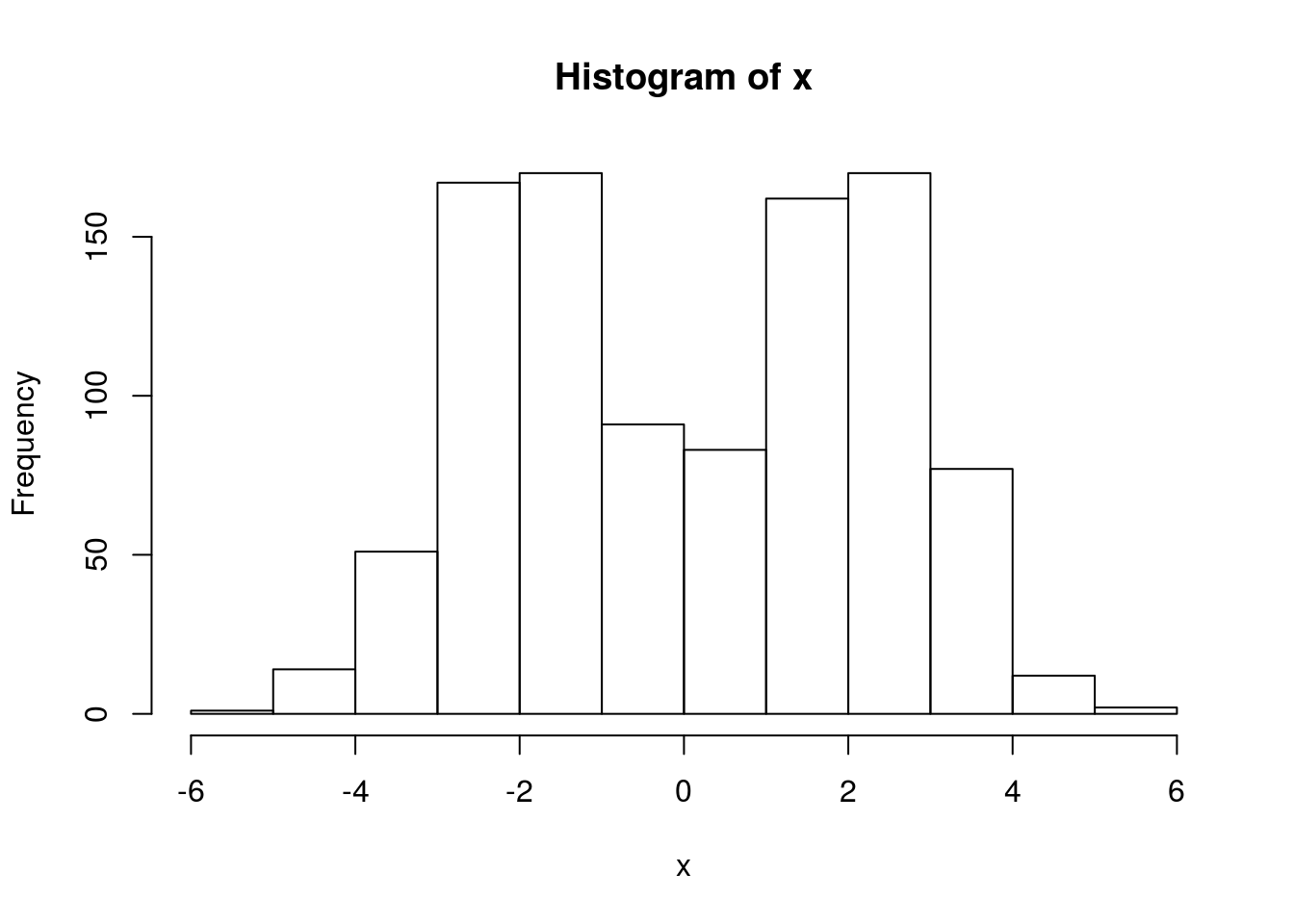
Gibbs sampler
Suppose we want to inference for the parameters \(\mu,\pi\). That is, we want to sample from \(p(\mu,\pi | x)\). We can use a Gibbs sampler. However, to do this we have to augment the space to sample from \(p(z,\mu,\pi | x)\), not only \(p(\mu,\pi | x)\).
Here is the algorithm in outline:
- sample \(\mu\) from \(\mu | x, z, \pi\)
- sample \(\pi\) from \(\pi | x, z, \mu\)
- sample \(z\) from \(z | x, \pi, \mu\)
The point here is that all of these conditionals are easy to sample from.
Code
  normalize = function(x){return(x/sum(x))}

  #' @param x an n vector of data
  #' @param pi a k vector
  #' @param mu a k vector
  sample_z = function(x,pi,mu){
    dmat = outer(mu,x,"-") # k by n matrix, d_kj =(mu_k - x_j)
    p.z.given.x = as.vector(pi) * dnorm(dmat,0,1)
    p.z.given.x = apply(p.z.given.x,2,normalize) # normalize columns
    z = rep(0, length(x))
    for(i in 1:length(z)){
      z[i] = sample(1:length(pi), size=1,prob=p.z.given.x[,i],replace=TRUE)
    }
    return(z)
  }


  #' @param z an n vector of cluster allocations (1...k)
  #' @param k the number of clusters
  sample_pi = function(z,k){
    counts = colSums(outer(z,1:k,FUN="=="))
    pi = gtools::rdirichlet(1,counts+1)
    return(pi)
  }

  #' @param x an n vector of data
  #' @param z an n vector of cluster allocations
  #' @param k the number o clusters
  #' @param prior.mean the prior mean for mu
  #' @param prior.prec the prior precision for mu
  sample_mu = function(x, z, k, prior){
    df = data.frame(x=x,z=z)
    mu = rep(0,k)
    for(i in 1:k){
      sample.size = sum(z==i)
      sample.mean = ifelse(sample.size==0,0,mean(x[z==i]))

      post.prec = sample.size+prior$prec
      post.mean = (prior$mean * prior$prec + sample.mean * sample.size)/post.prec
      mu[i] = rnorm(1,post.mean,sqrt(1/post.prec))
    }
    return(mu)
  }

  gibbs = function(x,k,niter =1000,muprior = list(mean=0,prec=0.1)){
    pi = rep(1/k,k) # initialize
    mu = rnorm(k,0,10)
    z = sample_z(x,pi,mu)
    res = list(mu=matrix(nrow=niter, ncol=k), pi = matrix(nrow=niter,ncol=k), z = matrix(nrow=niter, ncol=length(x)))
    res$mu[1,]=mu
    res$pi[1,]=pi
    res$z[1,]=z
    for(i in 2:niter){
        pi = sample_pi(z,k)
        mu = sample_mu(x,z,k,muprior)
        z = sample_z(x,pi,mu)
        res$mu[i,] = mu
        res$pi[i,] = pi
        res$z[i,] = z
    }
    return(res)
  }
Try the Gibbs sampler on the data simulated above. We see it quickly moves to a part of the space where the mean parameters are near their true values (-2,2).
  res = gibbs(x,2)
  plot(res$mu[,1],ylim=c(-4,4),type="l")
  lines(res$mu[,2],col=2)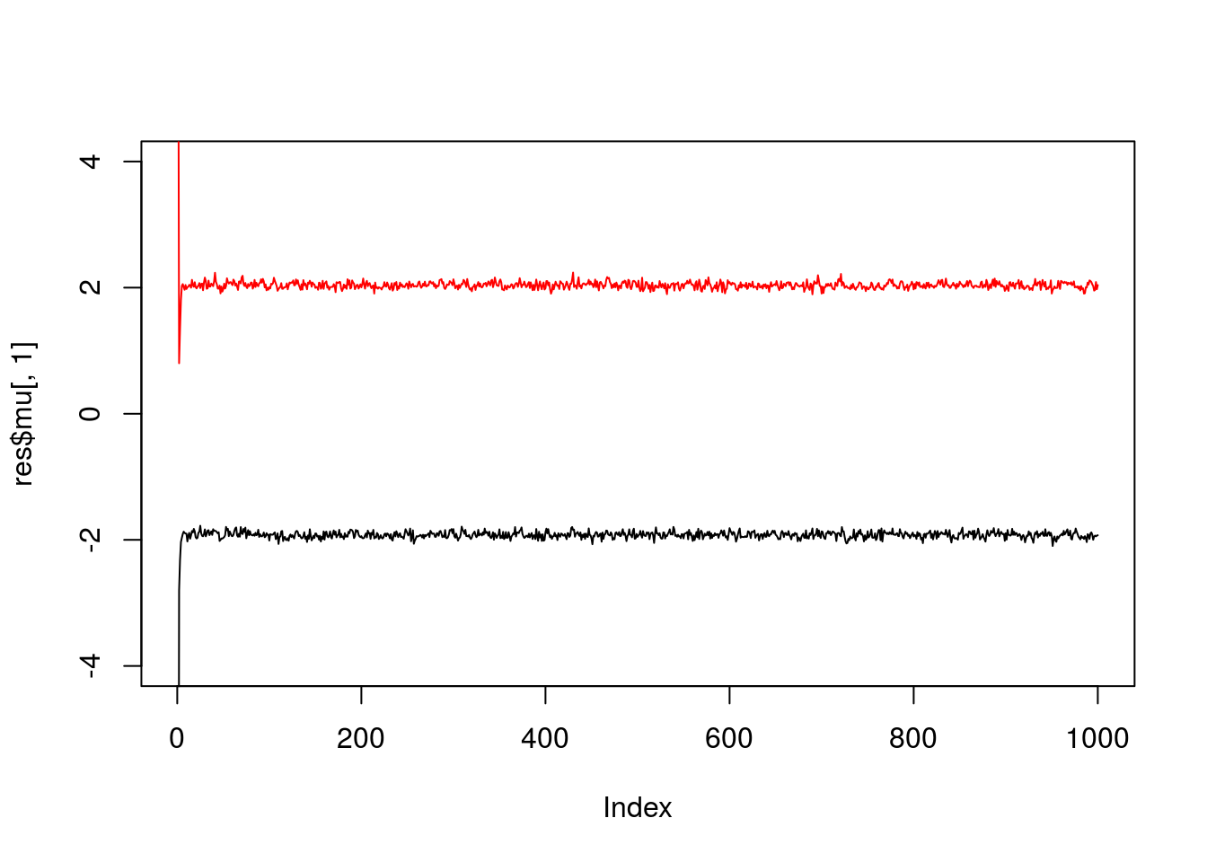
If we simulate data with fewer observations we should see more uncertainty
  x = rmix(100,c(0.5,0.5),c(-2,2),c(1,1))
  res2 = gibbs(x,2)
  plot(res2$mu[,1],ylim=c(-4,4),type="l")
  lines(res2$mu[,2],col=2)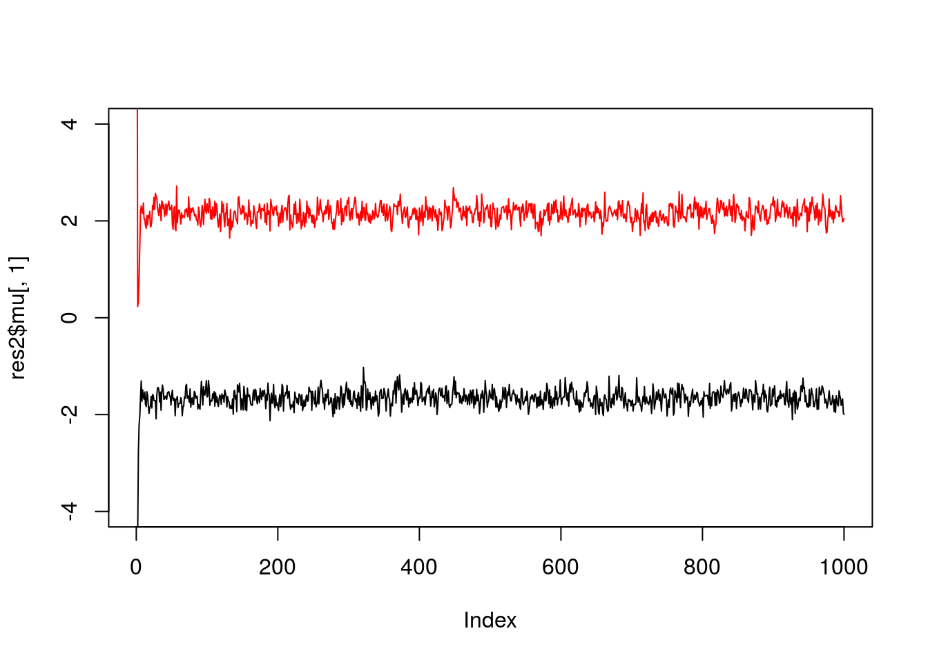
And fewer observations still…
  x = rmix(10,c(0.5,0.5),c(-2,2),c(1,1))
  res3 = gibbs(x,2)
  plot(res3$mu[,1],ylim=c(-4,4),type="l")
  lines(res3$mu[,2],col=2)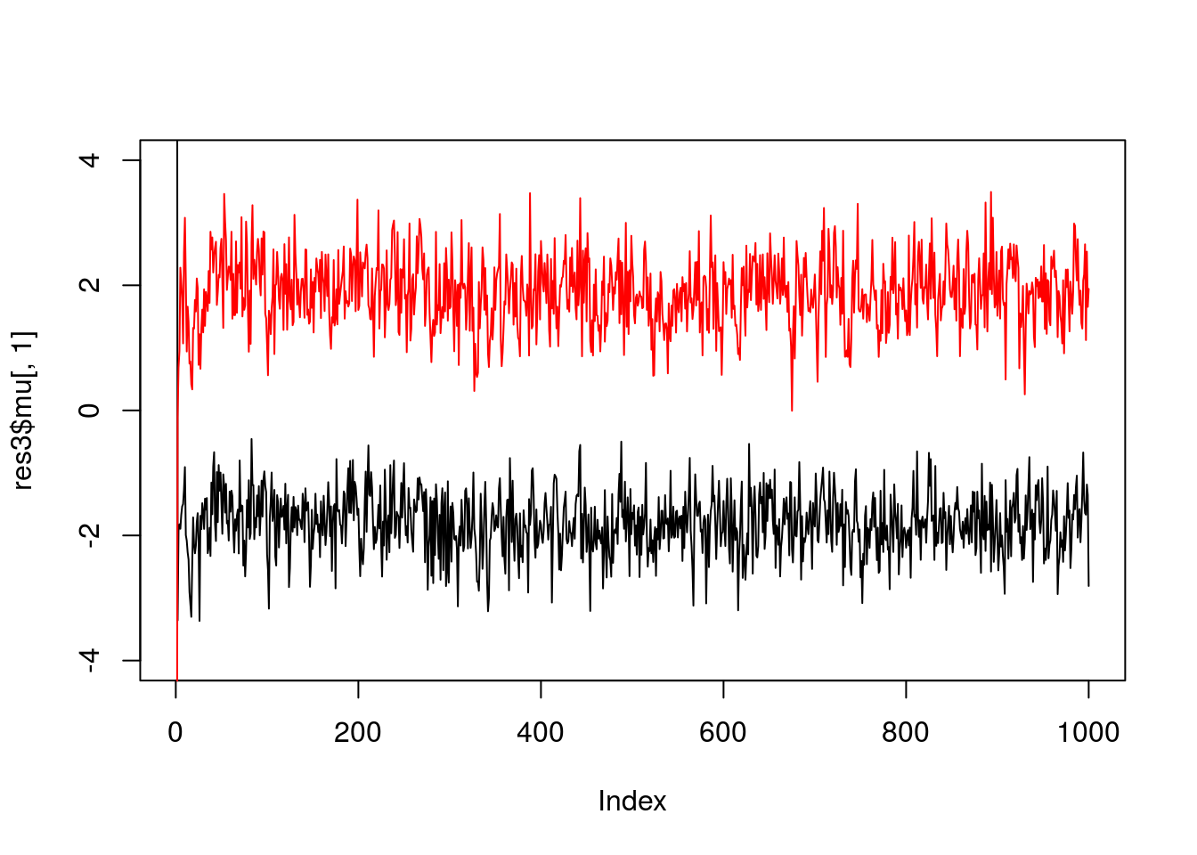
And we can get credible intervals (CI) from these samples (discard the first few samples as “burn-in”).
For example, to get 90% posterior CIs for the mean parameters:
quantile(res3$mu[-(1:10),1],c(0.05,0.95)) 5% 95%
-2.644896 -1.004009 quantile(res3$mu[-(1:10),2],c(0.05,0.95)) 5% 95%
0.9400428 2.7773584 Session information
sessionInfo()R version 3.3.2 (2016-10-31)
Platform: x86_64-pc-linux-gnu (64-bit)
Running under: Ubuntu 14.04.5 LTS
locale:
[1] LC_CTYPE=en_US.UTF-8 LC_NUMERIC=C
[3] LC_TIME=en_US.UTF-8 LC_COLLATE=en_US.UTF-8
[5] LC_MONETARY=en_US.UTF-8 LC_MESSAGES=en_US.UTF-8
[7] LC_PAPER=en_US.UTF-8 LC_NAME=C
[9] LC_ADDRESS=C LC_TELEPHONE=C
[11] LC_MEASUREMENT=en_US.UTF-8 LC_IDENTIFICATION=C
attached base packages:
[1] stats graphics grDevices utils datasets methods base
other attached packages:
[1] rmarkdown_1.1
loaded via a namespace (and not attached):
[1] magrittr_1.5 assertthat_0.1 formatR_1.4 htmltools_0.3.5
[5] tools_3.3.2 yaml_2.1.13 tibble_1.2 Rcpp_0.12.7
[9] stringi_1.1.1 knitr_1.14 stringr_1.0.0 digest_0.6.9
[13] gtools_3.5.0 evaluate_0.9 This site was created with R Markdown