Pre-requisites

Caveat on code

Note: the code here is designed to be readable by a beginner, rather than “efficient”. The idea is that you can use this code to learn about the basics of MCMC, but not as a model for how to program well in R!

Example 1: sampling from an exponential distribution using MCMC

Any MCMC scheme aims to produce (dependent) samples from a ``target" distribution. In this case we are going to use the exponential distribution with mean 1 as our target distribution. So we start by defining our target density:

target = function(x){
  if(x<0){
    return(0)}
  else {
    return( exp(-x))
  }
}

Having defined the function, we can now use it to compute a couple of values (just to illustrate the idea of a function):

target(1)

[1] 0.3678794

target(-1)

[1] 0

Next, we will program a Metropolis–Hastings scheme to sample from a distribution proportional to the target

x = rep(0,1000)
x[1] = 3     #this is just a starting value, which I've set arbitrarily to 3
for(i in 2:1000){
  currentx = x[i-1]
  proposedx = currentx + rnorm(1,mean=0,sd=1)
  A = target(proposedx)/target(currentx) 
  if(runif(1)<A){
    x[i] = proposedx       # accept move with probabily min(1,A)
  } else {
    x[i] = currentx        # otherwise "reject" move, and stay where we are
  }
}

Note that x is a realisation of a Markov Chain. We can make a few plots of x:

plot(x)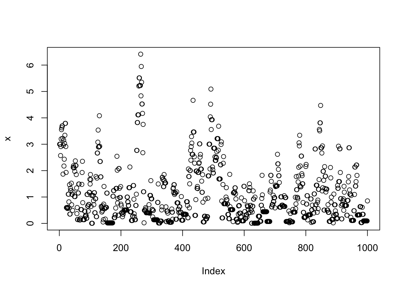 

hist(x)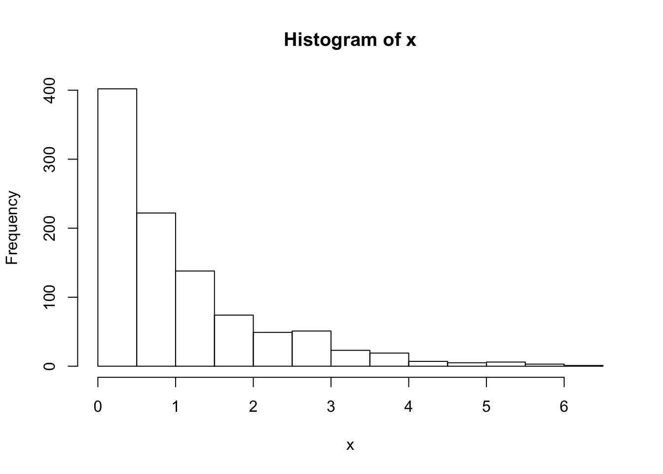

We can wrap this up in a function to make things a bit neater, and make it easy to try changing starting values and proposal distributions

easyMCMC = function(niter, startval, proposalsd){
  x = rep(0,niter)
  x[1] = startval     
  for(i in 2:niter){
    currentx = x[i-1]
    proposedx = rnorm(1,mean=currentx,sd=proposalsd) 
    A = target(proposedx)/target(currentx)
    if(runif(1)<A){
      x[i] = proposedx       # accept move with probabily min(1,A)
    } else {
      x[i] = currentx        # otherwise "reject" move, and stay where we are
    }
  }
  return(x)
}

Now we’ll run the MCMC scheme 3 times, and look to see how similar the results are:

z1=easyMCMC(1000,3,1)
z2=easyMCMC(1000,3,1)
z3=easyMCMC(1000,3,1)

plot(z1,type="l")
lines(z2,col=2)
lines(z3,col=3)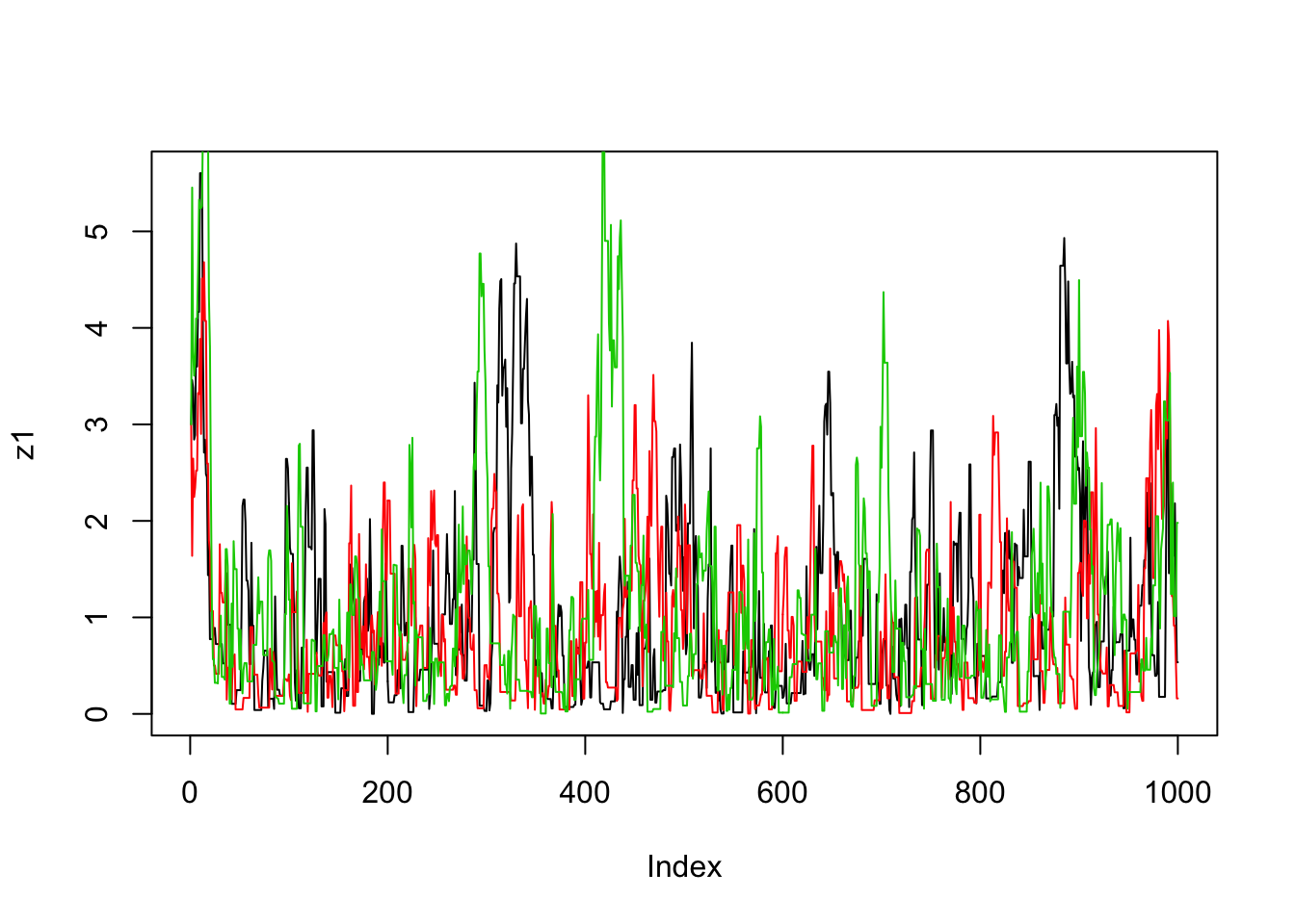

par(mfcol=c(3,1)) #rather odd command tells R to put 3 graphs on a single page
maxz=max(c(z1,z2,z3))
hist(z1,breaks=seq(0,maxz,length=20))
hist(z2,breaks=seq(0,maxz,length=20))
hist(z3,breaks=seq(0,maxz,length=20))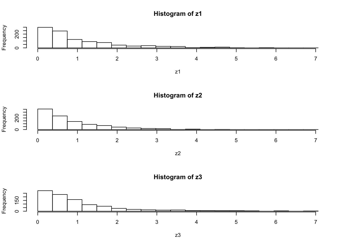

Exercises: use the function easyMCMC to explore the following: + 1a) how do different starting values affect the MCMC scheme?
+ 1b) what is the effect of having a bigger/smaller proposal standard deviation? + 1c) try changing the target function to the following

target = function(x){
  
  return((x>0 & x <1) + (x>2 & x<3))
}

What does this target look like? What happens if the proposal sd is too small here? (try eg 1 and 0.1)

Example 2: Estimating an allele frequency

A standard assumption when modelling genotypes of bi-allelic loci (eg loci with alleles A and a) is that the population is “randomly mating”. From this assumption it follows that the population will be in “Hardy Weinberg Equilibrium” (HWE), which means that if p is the frequency of the allele A then the genotypes AA, Aa and aa will have frequencies \(p^2, 2p(1-p)\) and \((1-p)^2\).

A simple prior for p is to assume it is uniform on [0,1]. Suppose that we sample n individuals, and observe nAA with genotype AA, nAa with genotype Aa and naa with genotype aa.

The following R code gives a short MCMC routine to sample from the posterior distribution of p. Try to go through the code to see how it works.

prior = function(p){
  if((p<0) || (p>1)){  # || here means "or"
    return(0)}
  else{
    return(1)}
}

likelihood = function(p, nAA, nAa, naa){
  return(p^(2*nAA) * (2*p*(1-p))^nAa * (1-p)^(2*naa))
}

psampler = function(nAA, nAa, naa, niter, pstartval, pproposalsd){
  p = rep(0,niter)
  p[1] = pstartval
  for(i in 2:niter){
    currentp = p[i-1]
    newp = currentp + rnorm(1,0,pproposalsd)
    A = prior(newp)*likelihood(newp,nAA,nAa,naa)/(prior(currentp) * likelihood(currentp,nAA,nAa,naa))
    if(runif(1)<A){
      p[i] = newp       # accept move with probabily min(1,A)
    } else {
      p[i] = currentp        # otherwise "reject" move, and stay where we are
    }
  }
  return(p)
}

Running this sample for nAA = 50, nAa = 21, naa=29.

z=psampler(50,21,29,10000,0.5,0.01)

Now some R code to compare the sample from the posterior with the theoretical posterior (which in this case is available analytically; since we observed 121 As, and 79 as, out of 200, the posterior for \(p\) is Beta(121+1,79+1).

x=seq(0,1,length=1000)
hist(z,prob=T)
lines(x,dbeta(x,122, 80))  # overlays beta density on histogram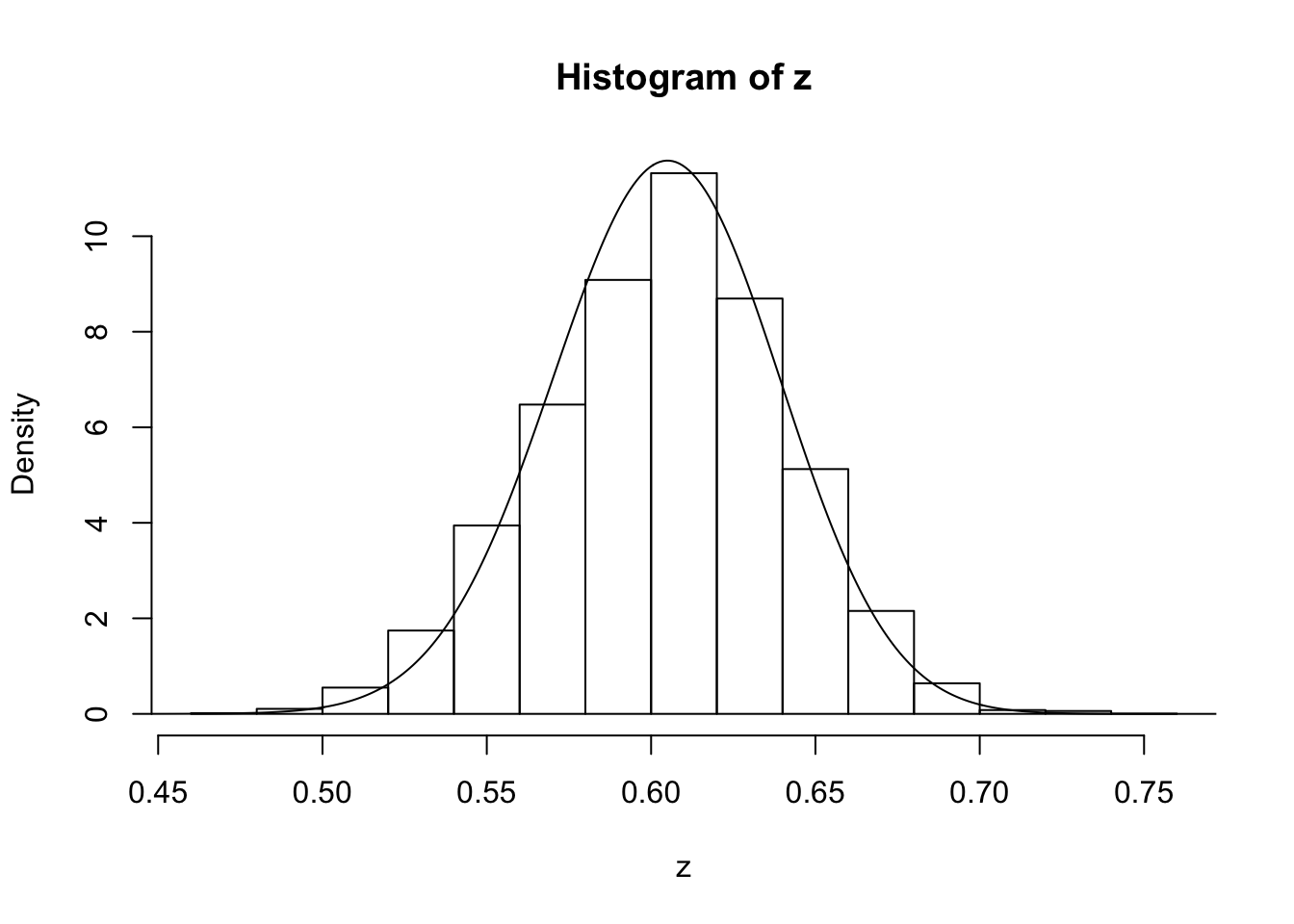

You might also like to discard the first 5000 z’s as “burnin”. Here’s one way in R to select only the last 5000 zs

hist(z[5001:10000])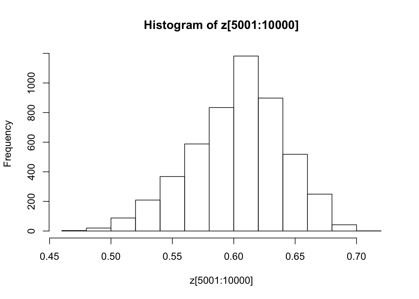

Some things to try: how do the starting point and proposal sd affect things?

Example 3: Estimating an allele frequency and inbreeding coefficient

A slightly more complex alternative than HWE is to assume that there is a tendency for people to mate with others who are slightly more closely-related than “random” (as might happen in a geographically-structured population, for example). This will result in an excess of homozygotes compared with HWE. A simple way to capture this is to introduce an extra parameter, the “inbreeding coefficient” f, and assume that the genotypes AA, Aa and aa have frequencies \(fp + (1-f)p*p, (1-f) 2p(1-p)\), and \(f(1-p) + (1-f)(1-p)(1-p)\).

In most cases it would be natural to treat f as a feature of the population, and therefore assume f is constant across loci. For simplicity we will consider just a single locus.

Note that both f and p are constrained to lie between 0 and 1 (inclusive). A simple prior for each of these two parameters is to assume that they are independent, uniform on [0,1]. Suppose that we sample n individuals, and observe nAA with genotype AA, nAa with genotype Aa and naa with genotype aa.

Exercise: write a short MCMC routine to sample from the joint distribution of f and p.

Hint: here is a start; you’ll need to fill in the …

fpsampler = function(nAA, nAa, naa, niter, fstartval, pstartval, fproposalsd, pproposalsd){
  f = rep(0,niter)
  p = rep(0,niter)
  f[1] = fstartval
  p[1] = pstartval
  for(i in 2:niter){
    currentf = f[i-1]
    currentp = p[i-1]
    newf = currentf + ...
    newp = currentp + ...
    ...
  }
  return(list(f=f,p=p)) # return a "list" with two elements named f and p
}

Addendum: Gibbs Sampling

You could also tackle this problem with a Gibbs Sampler (see vignettes here and here).

To do so you will want to use the following “latent variable” representation of the model: \[z_i \sim Bernoulli(f)\] \[p(g_i=AA | z_i=1) = p; p(g_i=AA | z_i=0) = p^2\] \[p(g_i=Aa | z_i = 1)= 0; p(g_i=Aa | z_i=0) = 2p(1-p)\] \[p(g_i=aa | z_i = 1) = (1-p); p(g_i =aa | z_i=0) = (1-p)^2\]

Summing over \(z_i\) gives the same model as above: \[p(g_i=AA) = fp + (1-f)p^2\]

Exercise: Implementing a Gibbs Sampler requires iterating the following steps 1) sample z from p(z | g, f, p) 2) sample f,p from p(f, p | g, z)

sessionInfo()

R version 3.3.2 (2016-10-31)
Platform: x86_64-apple-darwin13.4.0 (64-bit)
Running under: OS X El Capitan 10.11.6

locale:
[1] en_US.UTF-8/en_US.UTF-8/en_US.UTF-8/C/en_US.UTF-8/en_US.UTF-8

attached base packages:
[1] stats     graphics  grDevices utils     datasets  methods   base     

other attached packages:
[1] workflowr_0.3.0 rmarkdown_1.3  

loaded via a namespace (and not attached):
 [1] backports_1.0.5 magrittr_1.5    rprojroot_1.2   htmltools_0.3.5
 [5] tools_3.3.2     rstudioapi_0.6  yaml_2.1.14     Rcpp_0.12.8    
 [9] stringi_1.1.2   knitr_1.15.1    git2r_0.18.0    stringr_1.1.0  
[13] digest_0.6.10   evaluate_0.10