Normal Markov Chain
Matthew Stephens
2016-02-15
Last updated: 2017-01-02
Code version: 55e11cf8f7785ad926b716fb52e4e87b342f38e1
Pre-requisites
You should be familiar with the idea of a Markov chain, and with the multivariate normal distribution.
Overview
This vignette introduces the idea that in a multivariate normal, conditional independences correspond to the zeros of the precision matrix (inverse covariance matrix). It also prepares you for the idea of Brownian motion.
A normal markov chain
Consider a Markov chain \(X_1,X_2,X_3,\dots\) where the transitions are given by \(X_{t+1} | X_{t} \sim N(X_{t},1)\). You might think of this Markov chain as corresponding to a type of “random walk”: given the current state, the next state is obtained by adding a random normal with mean 0 and variance 1.
The following code simulates a realization of this Markov chain, starting from an initial state \(X_1 \sim N(0,1)\), and plots it.
set.seed(100)
sim_normal_MC=function(length=1000){
  X = rep(0,length)
  X[1] = rnorm(1)
  for(t in 2:length){
    X[t]= X[t-1] + rnorm(1)
  }
  return(X)
}
plot(sim_normal_MC())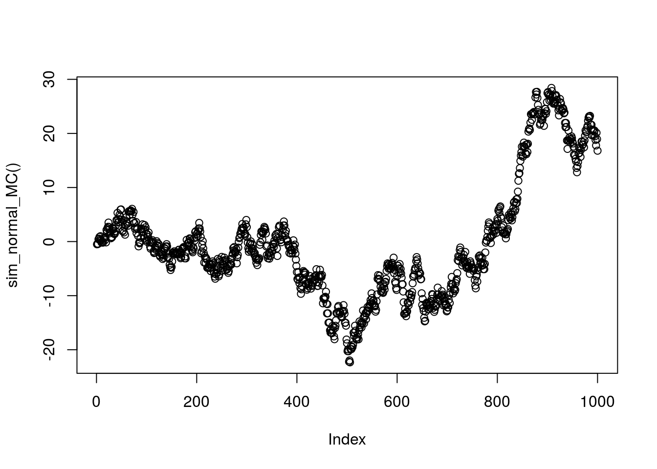
A normal markov chain as a multivariate normal
If you think a little you should be able to see that the above random walk simulation is actually simulating from a 1000-dimensional multivariate normal distribution!
Why?
Well, let’s write each of the \(N(0,1)\) variables we generate using ‘’rnorm’’ in that code as \(Z_1,Z_2,\dots\). Then: \[X_1 = Z_1\] \[X_2 = X_1 + Z_2 = Z_1 + Z_2\] \[X_3 = X_2 + Z_3 = Z_1 + Z_2 + Z_3\] etc.
So we can write \(X = AZ\) where \(A\) is the 1000 by 1000 matrix \[A = \begin{pmatrix} 1 & 0 & 0 & 0 & \dots \\ 1 & 1 & 0 & 0 & \dots \\ 1 & 1 & 1 & 0 & \dots \\ \dots \end{pmatrix}.\]
Let’s take a look at what the covariance matrix Sigma looks like. (We get a good idea from just looking at the top left corner of the matrix what the pattern is)
A = matrix(0,nrow=1000,ncol=1000)
for(i in 1:1000){
    A[i,]=c(rep(1,i),rep(0,1000-i))
}
Sigma = A %*% t(A)
Sigma[1:10,1:10]
[,1] [,2] [,3] [,4] [,5] [,6] [,7] [,8] [,9] [,10]
[1,] 1 1 1 1 1 1 1 1 1 1
[2,] 1 2 2 2 2 2 2 2 2 2
[3,] 1 2 3 3 3 3 3 3 3 3
[4,] 1 2 3 4 4 4 4 4 4 4
[5,] 1 2 3 4 5 5 5 5 5 5
[6,] 1 2 3 4 5 6 6 6 6 6
[7,] 1 2 3 4 5 6 7 7 7 7
[8,] 1 2 3 4 5 6 7 8 8 8
[9,] 1 2 3 4 5 6 7 8 9 9
[10,] 1 2 3 4 5 6 7 8 9 10Something interesting happens when we look at the inverse of this covariance matrix, which is referred to as the precision matrix, and often denoted \(\Omega\). Again we just show the top left corner of the precision matrix here.
Omega = chol2inv(chol(Sigma))
Omega[1:10,1:10]
[,1] [,2] [,3] [,4] [,5] [,6] [,7] [,8] [,9] [,10]
[1,] 2 -1 0 0 0 0 0 0 0 0
[2,] -1 2 -1 0 0 0 0 0 0 0
[3,] 0 -1 2 -1 0 0 0 0 0 0
[4,] 0 0 -1 2 -1 0 0 0 0 0
[5,] 0 0 0 -1 2 -1 0 0 0 0
[6,] 0 0 0 0 -1 2 -1 0 0 0
[7,] 0 0 0 0 0 -1 2 -1 0 0
[8,] 0 0 0 0 0 0 -1 2 -1 0
[9,] 0 0 0 0 0 0 0 -1 2 -1
[10,] 0 0 0 0 0 0 0 0 -1 2Notice all the 0s in the precision matrix. This is important! It is an example of the following much more general idea:
Let \(X\) be multivariate normal with covariance matrix \(\Sigma\) and precision matrix \(\Omega = \Sigma^{-1}\). Then \[\Omega_{ij}=0 \text{ if and only if } X_i \text{ and } X_j \text{ are conditionally independent given all other coordinates of } X.\]
Also, \[\Sigma_{ij}=0 \text{ if and only if } X_i \text{ and } X_j \text{ are independent}.\]
That is, the zeros of the covariance matrix tell us about independencies among coordinates of \(X\), and zeros of the precision matrix tell us about conditional independencies.
In a Markov chain (any Markov chain) the conditional distribution of \(X_t\) given the other \(X_s\) (\(s \neq t\)) depends only on its neighbors \(X_{t-1}\) and \(X_{t+1}\). That is, \(X_{t}\) is conditionally independent of all other \(X_s\) given \(X_{t-1}\) and \(X_{t+1}\). This is exactly what we are seeing in the precision matrix above: the non-zero elements of the \(t\)th row are at coordinates \(t-1,t\) and \(t+1\).
Session information
sessionInfo()R version 3.3.2 (2016-10-31)
Platform: x86_64-pc-linux-gnu (64-bit)
Running under: Ubuntu 14.04.5 LTS
locale:
[1] LC_CTYPE=en_US.UTF-8 LC_NUMERIC=C
[3] LC_TIME=en_US.UTF-8 LC_COLLATE=en_US.UTF-8
[5] LC_MONETARY=en_US.UTF-8 LC_MESSAGES=en_US.UTF-8
[7] LC_PAPER=en_US.UTF-8 LC_NAME=C
[9] LC_ADDRESS=C LC_TELEPHONE=C
[11] LC_MEASUREMENT=en_US.UTF-8 LC_IDENTIFICATION=C
attached base packages:
[1] stats graphics grDevices utils datasets methods base
other attached packages:
[1] MASS_7.3-45 expm_0.999-0 Matrix_1.2-7.1 rmarkdown_1.1
loaded via a namespace (and not attached):
[1] Rcpp_0.12.7 lattice_0.20-34 gtools_3.5.0 digest_0.6.9
[5] assertthat_0.1 grid_3.3.2 formatR_1.4 magrittr_1.5
[9] evaluate_0.9 stringi_1.1.1 tools_3.3.2 stringr_1.0.0
[13] yaml_2.1.13 htmltools_0.3.5 knitr_1.14 tibble_1.2 This site was created with R Markdown