Inverse Transform Sampling
Matt Bonakdarpour
2016-02-02
Last updated: 2019-03-31
Checks: 6 0
Knit directory: fiveMinuteStats/analysis/
This reproducible R Markdown analysis was created with workflowr (version 1.2.0). The Report tab describes the reproducibility checks that were applied when the results were created. The Past versions tab lists the development history.
Great! Since the R Markdown file has been committed to the Git repository, you know the exact version of the code that produced these results.
Great job! The global environment was empty. Objects defined in the global environment can affect the analysis in your R Markdown file in unknown ways. For reproduciblity it’s best to always run the code in an empty environment.
The command set.seed(12345) was run prior to running the code in the R Markdown file. Setting a seed ensures that any results that rely on randomness, e.g. subsampling or permutations, are reproducible.
Great job! Recording the operating system, R version, and package versions is critical for reproducibility.
Nice! There were no cached chunks for this analysis, so you can be confident that you successfully produced the results during this run.
Great! You are using Git for version control. Tracking code development and connecting the code version to the results is critical for reproducibility. The version displayed above was the version of the Git repository at the time these results were generated.
Note that you need to be careful to ensure that all relevant files for the analysis have been committed to Git prior to generating the results (you can use wflow_publish or wflow_git_commit). workflowr only checks the R Markdown file, but you know if there are other scripts or data files that it depends on. Below is the status of the Git repository when the results were generated:
Ignored files:
    Ignored:    .Rhistory
    Ignored:    .Rproj.user/
    Ignored:    analysis/.Rhistory
    Ignored:    analysis/bernoulli_poisson_process_cache/

Untracked files:
    Untracked:  _workflowr.yml
    Untracked:  analysis/CI.Rmd
    Untracked:  analysis/gibbs_structure.Rmd
    Untracked:  analysis/libs/
    Untracked:  analysis/results.Rmd
    Untracked:  analysis/shiny/tester/
    Untracked:  docs/MH_intro_files/
    Untracked:  docs/citations.bib
    Untracked:  docs/figure/MH_intro.Rmd/
    Untracked:  docs/figure/hmm.Rmd/
    Untracked:  docs/hmm_files/
    Untracked:  docs/libs/
    Untracked:  docs/shiny/tester/
Note that any generated files, e.g. HTML, png, CSS, etc., are not included in this status report because it is ok for generated content to have uncommitted changes.
These are the previous versions of the R Markdown and HTML files. If you’ve configured a remote Git repository (see ?wflow_git_remote), click on the hyperlinks in the table below to view them.
| File | Version | Author | Date | Message |
|---|---|---|---|---|
| Rmd | a86efa5 | Joseph Stachelek | 2018-04-25 | fix misspelling |
| html | 34bcc51 | John Blischak | 2017-03-06 | Build site. |
| Rmd | 5fbc8b5 | John Blischak | 2017-03-06 | Update workflowr project with wflow_update (version 0.4.0). |
| Rmd | 391ba3c | John Blischak | 2017-03-06 | Remove front and end matter of non-standard templates. |
| html | fb0f6e3 | stephens999 | 2017-03-03 | Merge pull request #33 from mdavy86/f/review |
| html | 0713277 | stephens999 | 2017-03-03 | Merge pull request #31 from mdavy86/f/review |
| Rmd | d674141 | Marcus Davy | 2017-02-27 | typos, refs |
| html | c3b365a | John Blischak | 2017-01-02 | Build site. |
| Rmd | 67a8575 | John Blischak | 2017-01-02 | Use external chunk to set knitr chunk options. |
| Rmd | 5ec12c7 | John Blischak | 2017-01-02 | Use session-info chunk. |
| Rmd | dfaabc4 | mbonakda | 2016-02-02 | spin off inverse transform sampling into its own note |
Pre-requisites
This document assumes basic familiarity with probability theory.
Overview
Inverse transform sampling is a method for generating random numbers from any probability distribution by using its inverse cumulative distribution \(F^{-1}(x)\). Recall that the cumulative distribution for a random variable \(X\) is \(F_X(x) = P(X \leq x)\). In what follows, we assume that our computer can, on demand, generate independent realizations of a random variable \(U\) uniformly distributed on \([0,1]\).
Algorithm
Continuous Distributions
Assume we want to generate a random variable \(X\) with cumulative distribution function (CDF) \(F_X\). The inverse transform sampling algorithm is simple:
1. Generate \(U \sim \text{Unif}(0,1)\)
2. Let \(X = F_X^{-1}(U)\).
Then, \(X\) will follow the distribution governed by the CDF \(F_X\), which was our desired result.
Note that this algorithm works in general but is not always practical. For example, inverting \(F_X\) is easy if \(X\) is an exponential random variable, but its harder if \(X\) is Normal random variable.
Discrete Distributions
Now we will consider the discrete version of the inverse transform method. Assume that \(X\) is a discrete random variable such that \(P(X = x_i) = p_i\). The algorithm proceeds as follows:
1. Generate \(U \sim \text{Unif}(0,1)\)
2. Determine the index \(k\) such that \(\sum_{j=1}^{k-1} p_j \leq U < \sum_{j=1}^k p_j\), and return \(X = x_k\).
Notice that the second step requires a search.
Assume our random variable \(X\) can take on any one of \(K\) values with probabilities \(\{p_1, \ldots, p_K\}\). We implement the algorithm below, assuming these probabilities are stored in a vector called p.vec.
# note: this inefficient implementation is for pedagogical purposes
# in general, consider using the rmultinom() function
discrete.inv.transform.sample <- function( p.vec ) {
  U  <- runif(1)
  if(U <= p.vec[1]){
    return(1)
  }
  for(state in 2:length(p.vec)) {
    if(sum(p.vec[1:(state-1)]) < U && U <= sum(p.vec[1:state]) ) {
      return(state)
    }
  }
}
Continuous Example: Exponential Distribution
Assume \(Y\) is an exponential random variable with rate parameter \(\lambda = 2\). Recall that the probability density function is \(p(y) = 2e^{-2y}\), for \(y > 0\). First, we compute the CDF: \[F_Y(x) = P(Y\leq x) = \int_0^x 2e^{-2y} dy = 1 - e^{-2x}\]
Solving for the inverse CDF, we get that \[F_Y^{-1}(y) = -\frac{\ln(1-y)}{2}\]
Using our algorithm above, we first generate \(U \sim \text{Unif}(0,1)\), then set \(X = F_Y^{-1}(U) = -\frac{\ln(1-U)}{2}\). We do this in the R code below and compare the histogram of our samples with the true density of \(Y\).
# inverse transform sampling
num.samples <-  1000
U           <-  runif(num.samples)
X           <- -log(1-U)/2

# plot
hist(X, freq=F, xlab='X', main='Generating Exponential R.V.')
curve(dexp(x, rate=2) , 0, 3, lwd=2, xlab = "", ylab = "", add = T)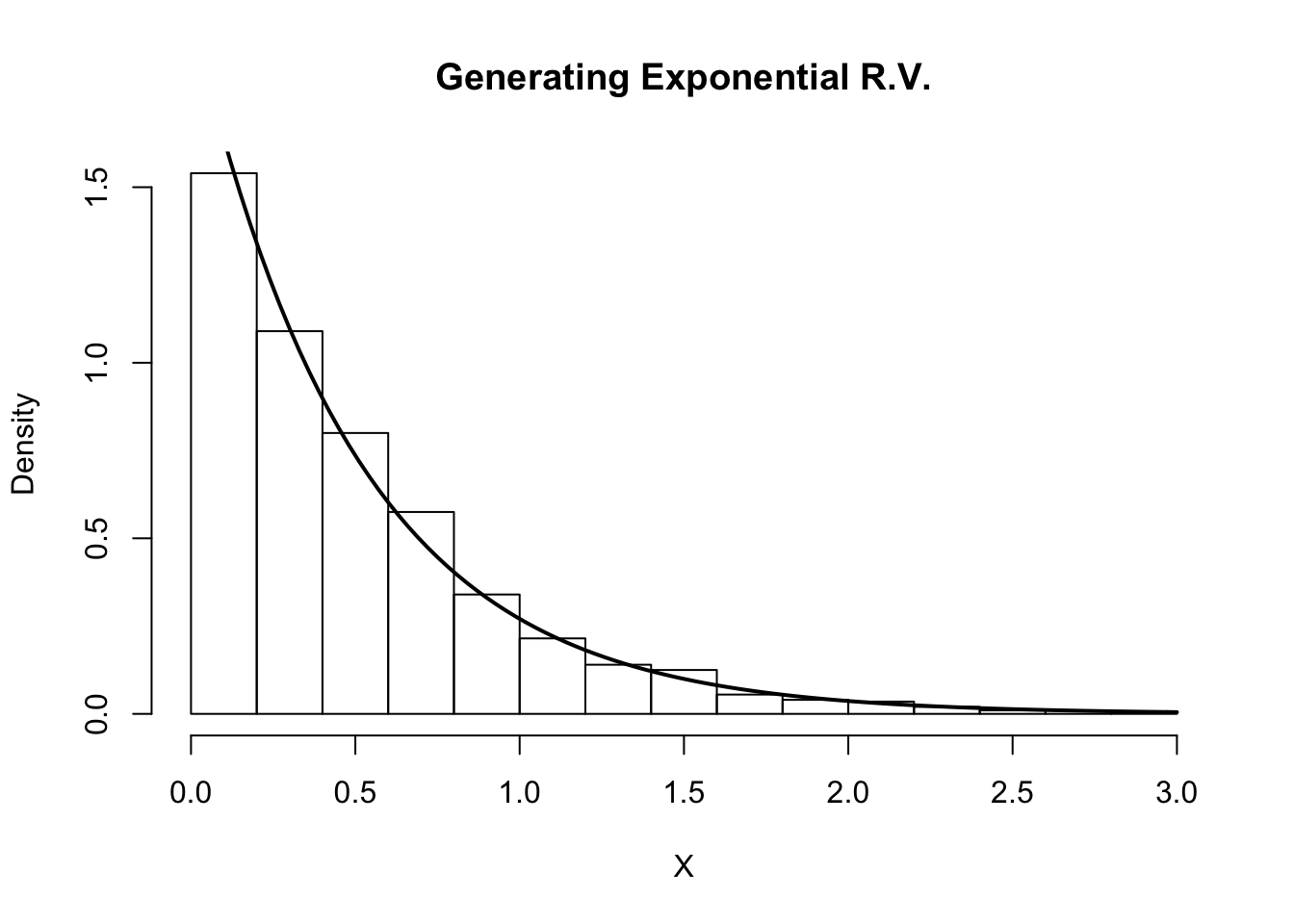
| Version | Author | Date |
|---|---|---|
| c3b365a | John Blischak | 2017-01-02 |
Indeed, the plot indicates that our random variables are following the intended distribution.
Discrete Example
Let’s assume we want to simulate a discrete random variable \(X\) that follows the following distribution:
| x_i | P(X=x_i) |
|---|---|
| 1 | 0.1 |
| 2 | 0.4 |
| 3 | 0.2 |
| 4 | 0.3 |
Below we simulate from this distribution using the discrete.inv.transform.sample() function above, and plot both the true probability vector, and the empirical proportions from our simulation.
num.samples <- 1000
p.vec        <- c(0.1, 0.4, 0.2, 0.3)
names(p.vec) <- 1:4
samples     <- numeric(num.samples)
for(i in seq_len(num.samples) ) {
  samples[i] <- discrete.inv.transform.sample(p.vec)
}
barplot(p.vec, main='True Probability Mass Function')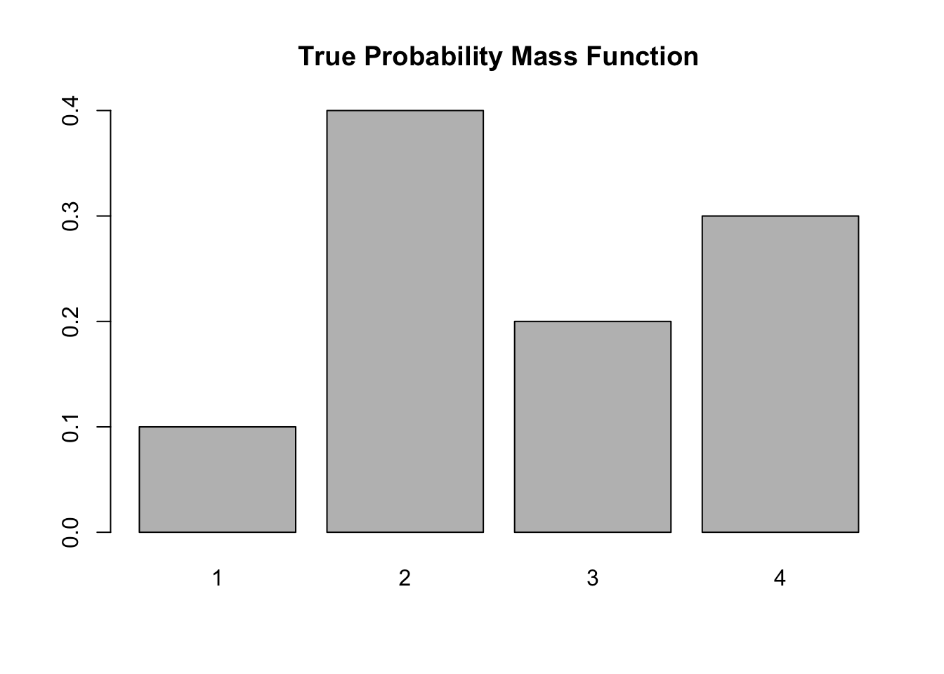
| Version | Author | Date |
|---|---|---|
| c3b365a | John Blischak | 2017-01-02 |
barplot(table(samples), main='Empirical Probability Mass Function')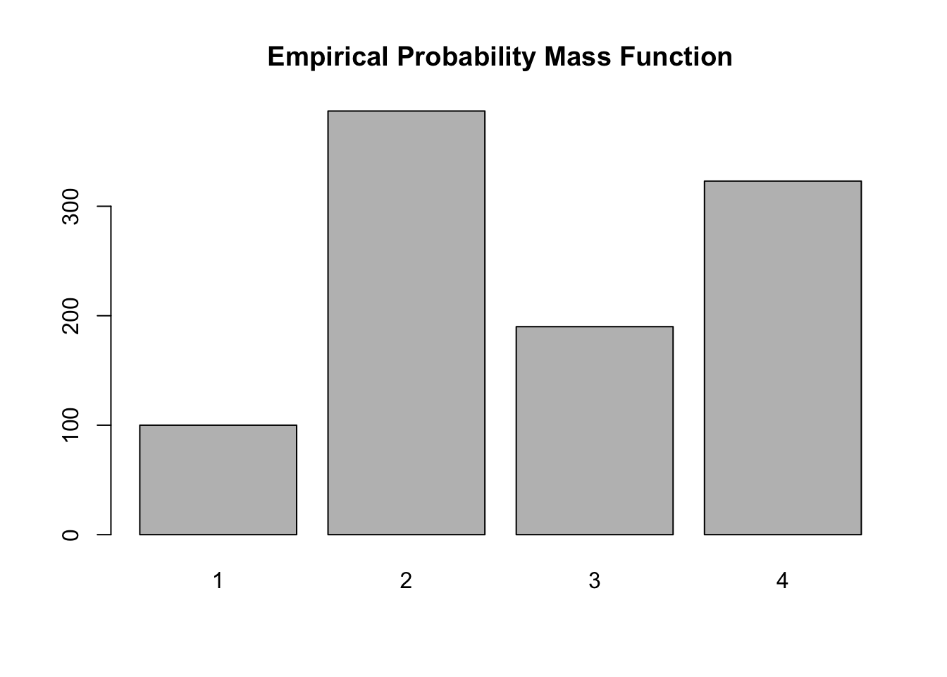
| Version | Author | Date |
|---|---|---|
| c3b365a | John Blischak | 2017-01-02 |
Again, the plot supports our claim that we are drawing from the true probability distribution
sessionInfo()R version 3.5.2 (2018-12-20)
Platform: x86_64-apple-darwin15.6.0 (64-bit)
Running under: macOS Mojave 10.14.1
Matrix products: default
BLAS: /Library/Frameworks/R.framework/Versions/3.5/Resources/lib/libRblas.0.dylib
LAPACK: /Library/Frameworks/R.framework/Versions/3.5/Resources/lib/libRlapack.dylib
locale:
[1] en_US.UTF-8/en_US.UTF-8/en_US.UTF-8/C/en_US.UTF-8/en_US.UTF-8
attached base packages:
[1] stats graphics grDevices utils datasets methods base
loaded via a namespace (and not attached):
[1] workflowr_1.2.0 Rcpp_1.0.0 digest_0.6.18 rprojroot_1.3-2
[5] backports_1.1.3 git2r_0.24.0 magrittr_1.5 evaluate_0.12
[9] stringi_1.2.4 fs_1.2.6 whisker_0.3-2 rmarkdown_1.11
[13] tools_3.5.2 stringr_1.3.1 glue_1.3.0 xfun_0.4
[17] yaml_2.2.0 compiler_3.5.2 htmltools_0.3.6 knitr_1.21 This site was created with R Markdown