Gibbs Sampling for clustering genetic data
Matthew Stephens
2017-02-20
Last updated: 2018-05-02
Code version: 8183f19
Pre-requisites
Be familiar with Bayesian inference for the two class problem and conjugate Bayesian analysis for a binomial proportion.
Overview
Suppose we observe genetic data on a sample of \(n\) elephants at \(R\) locations in the genome (“loci”). For simplicity we will assume the elephants are haploid: that is they have just one copy of their genome. And we will assume that there are just two genetic types (“alleles”) at each locus, which we will label 0 and 1.
We will further assume that there are two type of elephant: forest elephants and savanna elephants, and that the allele frequencies in forest elephants are different from those in savanna elephants, but that the allele frequencies for each of these two groups are unknown. Also, we do not know which samples are forest elephants and which are savanna elehants. Our goal is to infer both these sets of quantities: which individuals are forest vs savanna, and what are the allele frequencies in each group.
Notation
Let \(x_i\) denote the genetic data for individual \(i\) (\(i = 1,\dots, n\)). Thus \(x_i\) is a binary vector (a vector of 0s and 1s) of length \(R\). Let \(X\) denote the combined genetic data, \(X=(x_1,\dots,x_n)\).
Let \(z_i \in \{0,1\}\) denote the group (forest vs savanna) of individual \(i\), and let \(Z\) denote the vector \(Z=(z_1,\dots,z_n)\).
Let \(P_{kj}\) denote the frequency of the “1” allele at locus \(j\) in group \(k\) (\(j =1,\dots,R\); \(k=0,1\)). (Here group 0 means forest and group 1 means savanna.) Let \(P_k\) denote the vector \((P_{k1}, \dots, P_{kR})\), and \(P\) denote all the unknown allele frequencies \(P=(P_0,P_1)\).
With this notation in place, we can state the problem: infer the unknowns \(Z\) and \(P\) from the observations \(X\).
Model
To perform Bayesian inference for \(Z\) and \(P\) we need to specify the likelihood \(p(X | Z, P)\) and a prior distribution \(p(Z,P)\).
Likelihood
For the likelihood, for each individual we will assume that if we knew its group of origin, and we knew the allele frequencies in each group, then the genetic data at different markers are independent draws from the relevant allele frequencies. This is exactly the model assumed here. In mathematical notation, we assume: \[p(x_i | z_i , P) = \prod_{j=1}^R P_{{z_i} j}^{x_{ij}}(1-P_{{z_i}j})^{(1-x_{ij})}.\] All the subscripts here make this a bit difficult to read. To make things easier to read we can replace \(z_i\) with \(k\), like this: \[p(x_i | z_i=k , P) = \prod_{j=1}^R P_{k j}^{x_{ij}}(1-P_{kj})^{(1-x_{ij})}.\]
We will further assume that the different individuals are independent: \[p(X | Z, P) = \prod_i p(x_i | z_i, P).\] This completes specification of the likelihood.
Prior
We will assume that \(P\) and \(Z\) are a priori independent, so \(p(P,Z) = p(P)p(Z)\). This assumption seems reasonable: before seeing the genetic data \(X\), telling you the allele frequencies in the two groups would not tell you anything about the group membership of each individual. (Of course, after seeing the genetic data \(X\), the allele frequencies would help classify the individuals, so \(P\) and \(Z\) are not going to be a posteriori independent. However, here we are concerned with the prior, not the posterior.)
For the prior on \(P\) we will further assume that the allele frequencies in each group at each locus are independent, so \(p(P) = \prod_k \prod_j p(P_{kj})\). This assumption could be improved, but at the cost of considerable extra complexity, and so we stick with independence for now. Also for simplicity we will assume a uniform prior distribution for \(P_{kj}\), so \(p(P_{kj})=1\).
For \(Z\) we will assume that the origin of each individual is independent, with an equal probability (0.5) of arising from each of the two groups. So \[p(Z) = \prod_{i=1}^n p(z_i),\] and \(p(z_i=k) = 0.5\). Again, this assumption could be improved, but we start here for simplicity.
Computation
Our goal is to compute (or sample from) the posterior distribution \(p(Z,P | X)\), which by Bayes Theorem is given by \[p(Z, P | X) \propto p(X | Z,P) p(Z,P).\]
\[\Pr(X_{ij} = a | Z_i = k) = p^a_{kj} (1-p)^(1-a)_{kj}\] where \(a \in \{0,1\}\).
One way to sample from this distribution is to implement a Gibbs sampler. This requires us to be able to do two things:
- sample from Z | P,X
- sample from P | Z,X
These are called the “full conditional distributions” for Z and P respectively. The use of the word “full” here indicates that they are conditional on everything else (ie the data and all the other parameters).
Full conditional for Z
We know that: \[p(Z| P,X) \propto p(Z,P,X) = \prod_i p(x_i | z_i, P) p(z_i) p(P)\]
So we see that the full conditional for \(Z=(z_1,\dots,z_n)\) factorizes over \(i\) into terms that depend only on \(z_i\) and not the other \(z\)s. That is, \[p(Z| P,X) \propto \prod_i f_i(z_i; x_i,P)\]
for some functions \(f_i\).
This implies that the \(z_i\) are conditionally independent given \(X,P\), which is extremely convenient as it means we can compute their conditional distribution by just computing the marginals.
\[p(Z_i = k | P,X) \propto p(x_i | z_i=k, P)\]
TODO: fill in derivation of the conditional for P
Simulate some data
To illustrate, let’s simulate data from this model:
set.seed(33)

# generate from mixture of normals
#' @param n number of samples
#' @param P a 2 by R matrix of allele frequencies
r_simplemix = function(n,P){
  R = ncol(P)
  z = sample(1:2,prob=c(0.5,0.5),size=n,replace=TRUE) #simulate z as 1 or 2
  x = matrix(nrow = n, ncol=R)
  for(i in 1:n){
    x[i,] = rbinom(R,rep(1,R),P[z[i],])
  }
  return(list(x=x,z=z))
}
P = rbind(c(0.5,0.5,0.5,0.5,0.5,0.5),c(0.001,0.999,0.001,0.999,0.001,0.999))
sim = r_simplemix(n=50,P)
x = sim$x
Gibbs sampler code
#' @param x an R vector of data
#' @param P a K by R matrix of allele frequencies
#' @return the log-likelihood for each of the K populations
log_pr_x_given_P = function(x,P){
  tP = t(P) #transpose P so tP is R by K
  return(colSums(x*log(tP)+(1-x)*log(1-tP)))
}

normalize = function(x){return(x/sum(x))} #used in sample_z below

#' @param x an n by R matrix of data
#' @param P a K by R matrix of allele frequencies
#' @return an n vector of group memberships
sample_z = function(x,P){
  K = nrow(P)
  loglik_matrix = apply(x, 1, log_pr_x_given_P, P=P)
  lik_matrix = exp(loglik_matrix)
  p.z.given.x = apply(lik_matrix,2,normalize) # normalize columns
  z = rep(0, nrow(x))
  for(i in 1:length(z)){
    z[i] = sample(1:K, size=1,prob=p.z.given.x[,i],replace=TRUE)
  }
  return(z)
}


#' @param x an n by R matrix of data
#' @param z an n vector of cluster allocations
#' @return a 2 by R matrix of allele frequencies
sample_P = function(x, z){
  R = ncol(x)
  P = matrix(ncol=R,nrow=2)
  for(i in 1:2){
    sample_size = sum(z==i)
    if(sample_size==0){
      number_of_ones=rep(0,R)
    } else {
      number_of_ones = colSums(x[z==i,])
    }
    P[i,] = rbeta(R,1+number_of_ones,1+sample_size-number_of_ones)
  }
  return(P)
}

gibbs = function(x,niter = 100){
  z = sample(1:2,nrow(x),replace=TRUE)
  res = list(z = matrix(nrow=niter, ncol=nrow(x)))
  res$z[1,]=z

  for(i in 2:niter){
    P = sample_P(x,z)
    z = sample_z(x,P)
    res$z[i,] = z
  }
  return(res)
}
Try the Gibbs sampler on the data simulated above.
  res = gibbs(x,100)
  table(res$z[1,],sim$z)
     1  2
  1 13 14
  2 11 12
table(res$z[100,],sim$z)
     1  2
  1  4 26
  2 20  0
image(t(res$z))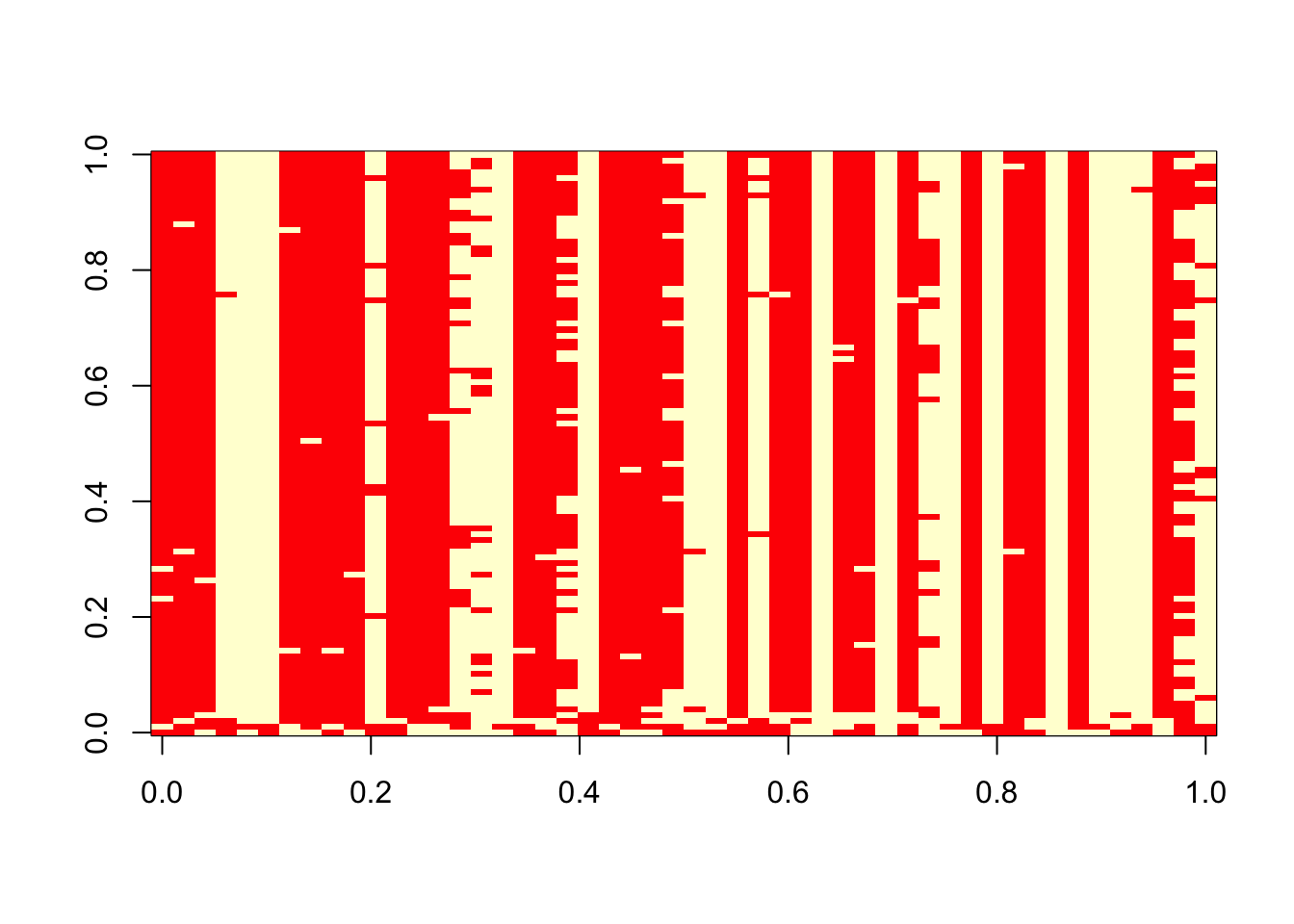
Session Information
sessionInfo()R version 3.3.2 (2016-10-31)
Platform: x86_64-apple-darwin13.4.0 (64-bit)
Running under: OS X El Capitan 10.11.6
locale:
[1] en_US.UTF-8/en_US.UTF-8/en_US.UTF-8/C/en_US.UTF-8/en_US.UTF-8
attached base packages:
[1] stats graphics grDevices utils datasets methods base
loaded via a namespace (and not attached):
[1] workflowr_1.0.1 Rcpp_0.12.16 digest_0.6.15
[4] rprojroot_1.3-2 R.methodsS3_1.7.1 backports_1.1.2
[7] git2r_0.21.0 magrittr_1.5 evaluate_0.10.1
[10] stringi_1.1.7 R.oo_1.22.0 R.utils_2.6.0
[13] rmarkdown_1.9 tools_3.3.2 stringr_1.3.0
[16] yaml_2.1.18 htmltools_0.3.6 knitr_1.20 This site was created with R Markdown