Gibbs Sampling for a mixture of normals
Matthew Stephens
2016-06-01
Last updated: 2019-03-31
Checks: 6 0
Knit directory: fiveMinuteStats/analysis/
This reproducible R Markdown analysis was created with workflowr (version 1.2.0). The Report tab describes the reproducibility checks that were applied when the results were created. The Past versions tab lists the development history.
Great! Since the R Markdown file has been committed to the Git repository, you know the exact version of the code that produced these results.
Great job! The global environment was empty. Objects defined in the global environment can affect the analysis in your R Markdown file in unknown ways. For reproduciblity it’s best to always run the code in an empty environment.
The command set.seed(12345) was run prior to running the code in the R Markdown file. Setting a seed ensures that any results that rely on randomness, e.g. subsampling or permutations, are reproducible.
Great job! Recording the operating system, R version, and package versions is critical for reproducibility.
Nice! There were no cached chunks for this analysis, so you can be confident that you successfully produced the results during this run.
Great! You are using Git for version control. Tracking code development and connecting the code version to the results is critical for reproducibility. The version displayed above was the version of the Git repository at the time these results were generated.
Note that you need to be careful to ensure that all relevant files for the analysis have been committed to Git prior to generating the results (you can use wflow_publish or wflow_git_commit). workflowr only checks the R Markdown file, but you know if there are other scripts or data files that it depends on. Below is the status of the Git repository when the results were generated:
Ignored files:
    Ignored:    .Rhistory
    Ignored:    .Rproj.user/
    Ignored:    analysis/.Rhistory
    Ignored:    analysis/bernoulli_poisson_process_cache/

Untracked files:
    Untracked:  _workflowr.yml
    Untracked:  analysis/CI.Rmd
    Untracked:  analysis/gibbs_structure.Rmd
    Untracked:  analysis/libs/
    Untracked:  analysis/results.Rmd
    Untracked:  analysis/shiny/tester/
    Untracked:  docs/MH_intro_files/
    Untracked:  docs/citations.bib
    Untracked:  docs/figure/MH_intro.Rmd/
    Untracked:  docs/hmm_files/
    Untracked:  docs/libs/
    Untracked:  docs/shiny/tester/
Note that any generated files, e.g. HTML, png, CSS, etc., are not included in this status report because it is ok for generated content to have uncommitted changes.
These are the previous versions of the R Markdown and HTML files. If you’ve configured a remote Git repository (see ?wflow_git_remote), click on the hyperlinks in the table below to view them.
| File | Version | Author | Date | Message |
|---|---|---|---|---|
| html | 34bcc51 | John Blischak | 2017-03-06 | Build site. |
| Rmd | 5fbc8b5 | John Blischak | 2017-03-06 | Update workflowr project with wflow_update (version 0.4.0). |
| Rmd | 391ba3c | John Blischak | 2017-03-06 | Remove front and end matter of non-standard templates. |
| html | fb0f6e3 | stephens999 | 2017-03-03 | Merge pull request #33 from mdavy86/f/review |
| html | c3b365a | John Blischak | 2017-01-02 | Build site. |
| Rmd | 67a8575 | John Blischak | 2017-01-02 | Use external chunk to set knitr chunk options. |
| Rmd | 5ec12c7 | John Blischak | 2017-01-02 | Use session-info chunk. |
| Rmd | a8c9d57 | stephens999 | 2016-09-04 | correct misleading names in gibbs2 example |
| Rmd | 6bb4560 | stephens999 | 2016-05-12 | add gibbs sampling example |
Pre-requisites
Know what a Gibbs sampler is, and a mixture model is, and be familiar with Bayesian inference for a normal mean and for the two class problem.
Overview
We consider using Gibbs sampling to perform inference for a normal mixture model, \[X_1,\dots,X_n \sim f(\cdot)\] where \[f(\cdot) = \sum_{k=1}^K \pi_k N(\cdot; \mu_k,1).\] Here \(\pi_1,\dots,\pi_K\) are non-negative and sum to 1, and \(N(\cdot;\mu,\sigma^2)\) denotes the density of the \(N(\mu,\sigma^2)\) distribution.
Recall the latent variable representation of this model: \[\Pr(Z_j = k) = \pi_k\] \[X_j | Z_j = k \sim N(\mu_k,1)\]
To illustrate, let’s simulate data from this model:
set.seed(33)

# generate from mixture of normals
#' @param n number of samples
#' @param pi mixture proportions
#' @param mu mixture means
#' @param s mixture standard deviations
rmix = function(n,pi,mu,s){
  z = sample(1:length(pi),prob=pi,size=n,replace=TRUE)
  x = rnorm(n,mu[z],s[z])
  return(x)
}
x = rmix(n=1000,pi=c(0.5,0.5),mu=c(-2,2),s=c(1,1))
hist(x)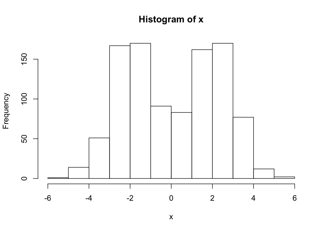
| Version | Author | Date |
|---|---|---|
| c3b365a | John Blischak | 2017-01-02 |
Gibbs sampler
Suppose we want to inference for the parameters \(\mu,\pi\). That is, we want to sample from \(p(\mu,\pi | x)\). We can use a Gibbs sampler. However, to do this we have to augment the space to sample from \(p(z,\mu,\pi | x)\), not only \(p(\mu,\pi | x)\).
Here is the algorithm in outline:
- sample \(\mu\) from \(\mu | x, z, \pi\)
- sample \(\pi\) from \(\pi | x, z, \mu\)
- sample \(z\) from \(z | x, \pi, \mu\)
The point here is that all of these conditionals are easy to sample from.
Code
  normalize = function(x){return(x/sum(x))}

  #' @param x an n vector of data
  #' @param pi a k vector
  #' @param mu a k vector
  sample_z = function(x,pi,mu){
    dmat = outer(mu,x,"-") # k by n matrix, d_kj =(mu_k - x_j)
    p.z.given.x = as.vector(pi) * dnorm(dmat,0,1)
    p.z.given.x = apply(p.z.given.x,2,normalize) # normalize columns
    z = rep(0, length(x))
    for(i in 1:length(z)){
      z[i] = sample(1:length(pi), size=1,prob=p.z.given.x[,i],replace=TRUE)
    }
    return(z)
  }


  #' @param z an n vector of cluster allocations (1...k)
  #' @param k the number of clusters
  sample_pi = function(z,k){
    counts = colSums(outer(z,1:k,FUN="=="))
    pi = gtools::rdirichlet(1,counts+1)
    return(pi)
  }

  #' @param x an n vector of data
  #' @param z an n vector of cluster allocations
  #' @param k the number o clusters
  #' @param prior.mean the prior mean for mu
  #' @param prior.prec the prior precision for mu
  sample_mu = function(x, z, k, prior){
    df = data.frame(x=x,z=z)
    mu = rep(0,k)
    for(i in 1:k){
      sample.size = sum(z==i)
      sample.mean = ifelse(sample.size==0,0,mean(x[z==i]))

      post.prec = sample.size+prior$prec
      post.mean = (prior$mean * prior$prec + sample.mean * sample.size)/post.prec
      mu[i] = rnorm(1,post.mean,sqrt(1/post.prec))
    }
    return(mu)
  }

  gibbs = function(x,k,niter =1000,muprior = list(mean=0,prec=0.1)){
    pi = rep(1/k,k) # initialize
    mu = rnorm(k,0,10)
    z = sample_z(x,pi,mu)
    res = list(mu=matrix(nrow=niter, ncol=k), pi = matrix(nrow=niter,ncol=k), z = matrix(nrow=niter, ncol=length(x)))
    res$mu[1,]=mu
    res$pi[1,]=pi
    res$z[1,]=z
    for(i in 2:niter){
        pi = sample_pi(z,k)
        mu = sample_mu(x,z,k,muprior)
        z = sample_z(x,pi,mu)
        res$mu[i,] = mu
        res$pi[i,] = pi
        res$z[i,] = z
    }
    return(res)
  }
Try the Gibbs sampler on the data simulated above. We see it quickly moves to a part of the space where the mean parameters are near their true values (-2,2).
  res = gibbs(x,2)
  plot(res$mu[,1],ylim=c(-4,4),type="l")
  lines(res$mu[,2],col=2)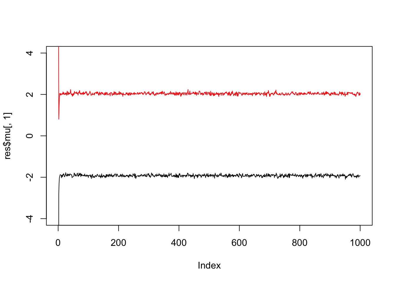
| Version | Author | Date |
|---|---|---|
| c3b365a | John Blischak | 2017-01-02 |
If we simulate data with fewer observations we should see more uncertainty
  x = rmix(100,c(0.5,0.5),c(-2,2),c(1,1))
  res2 = gibbs(x,2)
  plot(res2$mu[,1],ylim=c(-4,4),type="l")
  lines(res2$mu[,2],col=2)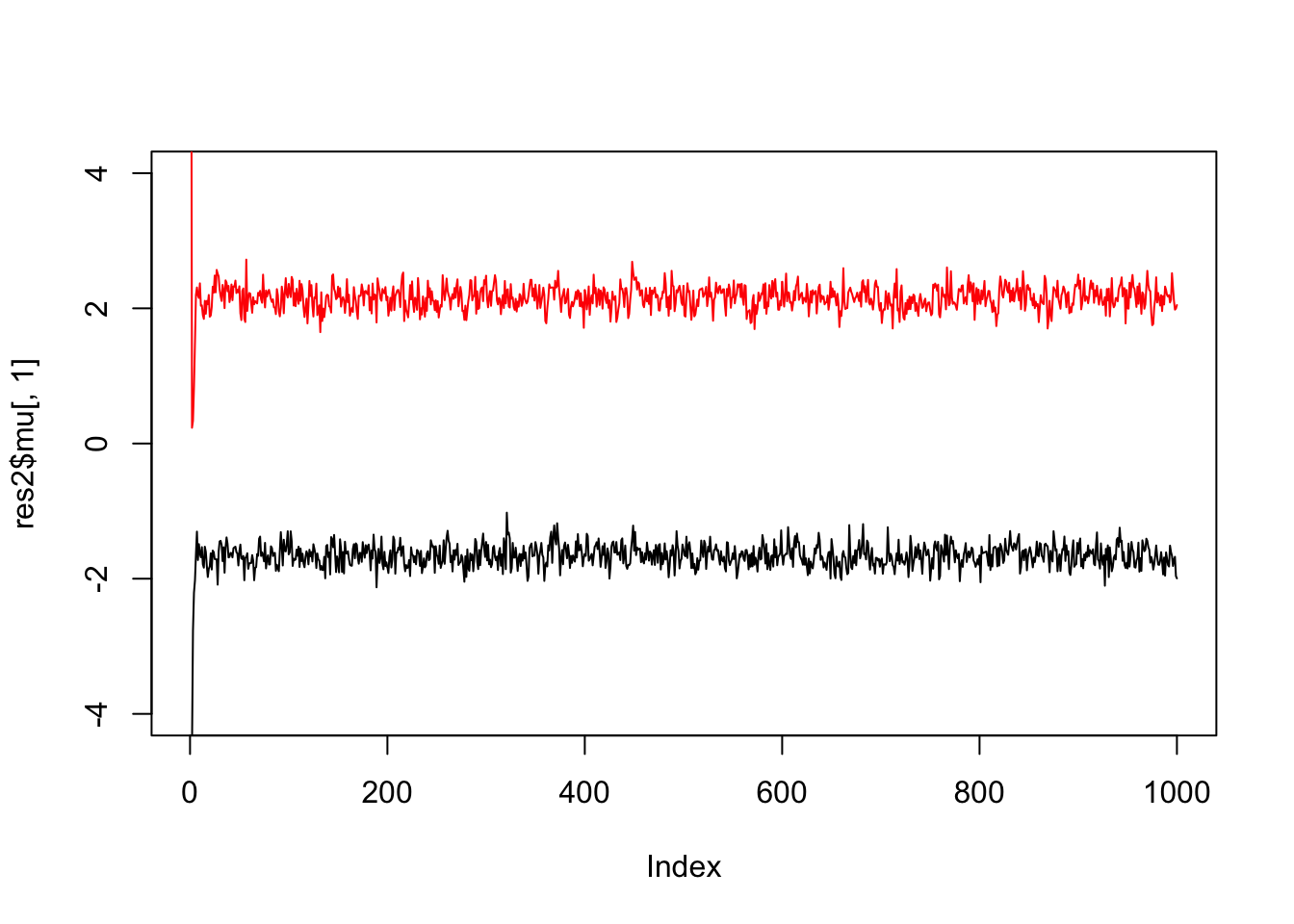
| Version | Author | Date |
|---|---|---|
| c3b365a | John Blischak | 2017-01-02 |
And fewer observations still…
  x = rmix(10,c(0.5,0.5),c(-2,2),c(1,1))
  res3 = gibbs(x,2)
  plot(res3$mu[,1],ylim=c(-4,4),type="l")
  lines(res3$mu[,2],col=2)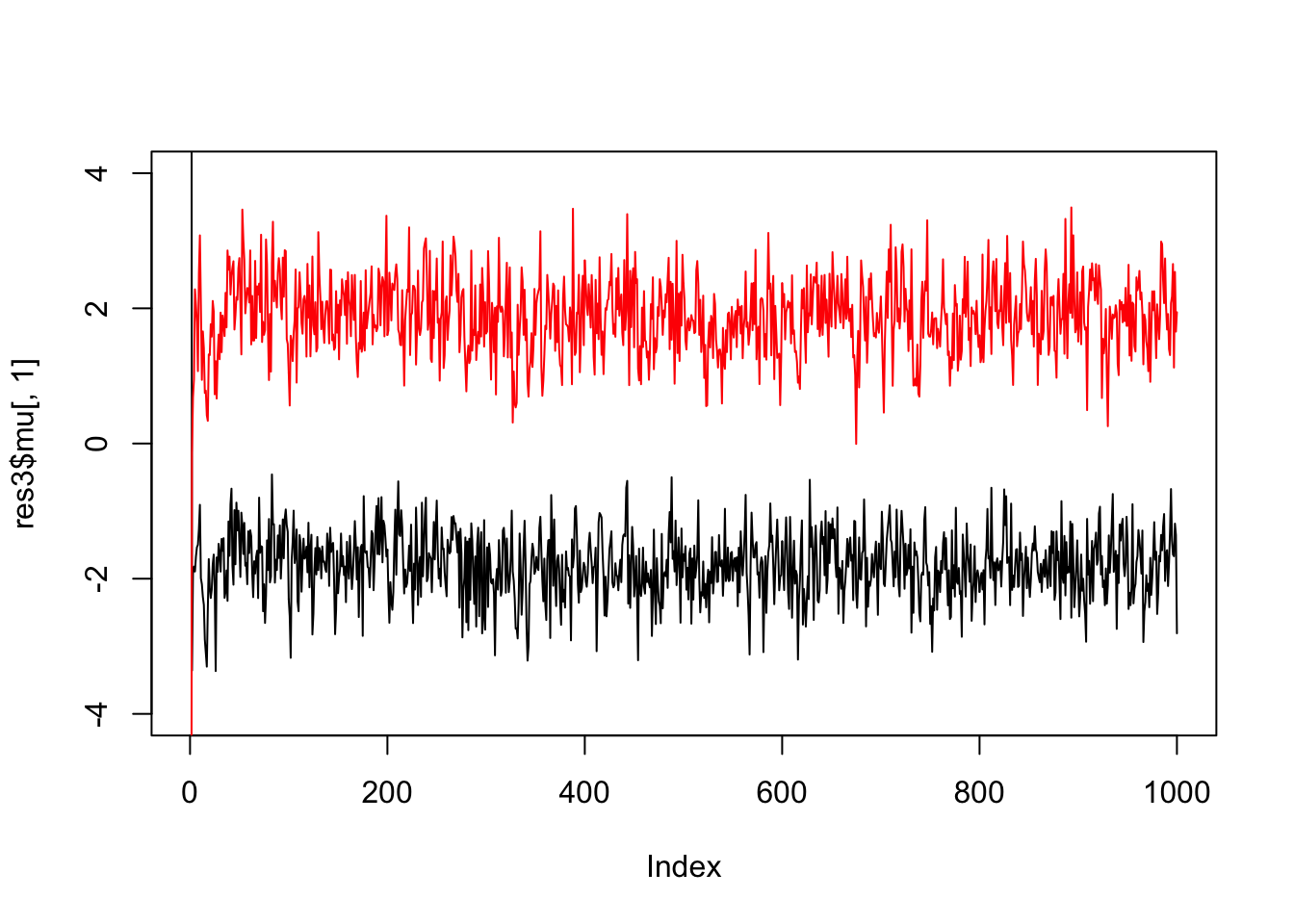
| Version | Author | Date |
|---|---|---|
| c3b365a | John Blischak | 2017-01-02 |
And we can get credible intervals (CI) from these samples (discard the first few samples as “burn-in”).
For example, to get 90% posterior CIs for the mean parameters:
quantile(res3$mu[-(1:10),1],c(0.05,0.95)) 5% 95%
-2.644896 -1.004009 quantile(res3$mu[-(1:10),2],c(0.05,0.95)) 5% 95%
0.9400428 2.7773584
sessionInfo()R version 3.5.2 (2018-12-20)
Platform: x86_64-apple-darwin15.6.0 (64-bit)
Running under: macOS Mojave 10.14.1
Matrix products: default
BLAS: /Library/Frameworks/R.framework/Versions/3.5/Resources/lib/libRblas.0.dylib
LAPACK: /Library/Frameworks/R.framework/Versions/3.5/Resources/lib/libRlapack.dylib
locale:
[1] en_US.UTF-8/en_US.UTF-8/en_US.UTF-8/C/en_US.UTF-8/en_US.UTF-8
attached base packages:
[1] stats graphics grDevices utils datasets methods base
loaded via a namespace (and not attached):
[1] workflowr_1.2.0 Rcpp_1.0.0 gtools_3.8.1 digest_0.6.18
[5] rprojroot_1.3-2 backports_1.1.3 git2r_0.24.0 magrittr_1.5
[9] evaluate_0.12 stringi_1.2.4 fs_1.2.6 whisker_0.3-2
[13] rmarkdown_1.11 tools_3.5.2 stringr_1.3.1 glue_1.3.0
[17] xfun_0.4 yaml_2.2.0 compiler_3.5.2 htmltools_0.3.6
[21] knitr_1.21 This site was created with R Markdown