The likelihood ratio for continuous data
Matthew Stephens
2016-01-07
Last updated: 2019-03-31
Checks: 6 0
Knit directory: fiveMinuteStats/analysis/
This reproducible R Markdown analysis was created with workflowr (version 1.2.0). The Report tab describes the reproducibility checks that were applied when the results were created. The Past versions tab lists the development history.
Great! Since the R Markdown file has been committed to the Git repository, you know the exact version of the code that produced these results.
Great job! The global environment was empty. Objects defined in the global environment can affect the analysis in your R Markdown file in unknown ways. For reproduciblity it’s best to always run the code in an empty environment.
The command set.seed(12345) was run prior to running the code in the R Markdown file. Setting a seed ensures that any results that rely on randomness, e.g. subsampling or permutations, are reproducible.
Great job! Recording the operating system, R version, and package versions is critical for reproducibility.
Nice! There were no cached chunks for this analysis, so you can be confident that you successfully produced the results during this run.
Great! You are using Git for version control. Tracking code development and connecting the code version to the results is critical for reproducibility. The version displayed above was the version of the Git repository at the time these results were generated.
Note that you need to be careful to ensure that all relevant files for the analysis have been committed to Git prior to generating the results (you can use wflow_publish or wflow_git_commit). workflowr only checks the R Markdown file, but you know if there are other scripts or data files that it depends on. Below is the status of the Git repository when the results were generated:
Ignored files:
    Ignored:    .Rhistory
    Ignored:    .Rproj.user/
    Ignored:    analysis/.Rhistory
    Ignored:    analysis/bernoulli_poisson_process_cache/

Untracked files:
    Untracked:  _workflowr.yml
    Untracked:  analysis/CI.Rmd
    Untracked:  analysis/gibbs_structure.Rmd
    Untracked:  analysis/libs/
    Untracked:  analysis/results.Rmd
    Untracked:  analysis/shiny/tester/
    Untracked:  docs/MH_intro_files/
    Untracked:  docs/citations.bib
    Untracked:  docs/figure/MH_intro.Rmd/
    Untracked:  docs/figure/hmm.Rmd/
    Untracked:  docs/hmm_files/
    Untracked:  docs/libs/
    Untracked:  docs/shiny/tester/
Note that any generated files, e.g. HTML, png, CSS, etc., are not included in this status report because it is ok for generated content to have uncommitted changes.
These are the previous versions of the R Markdown and HTML files. If you’ve configured a remote Git repository (see ?wflow_git_remote), click on the hyperlinks in the table below to view them.
| File | Version | Author | Date | Message |
|---|---|---|---|---|
| html | 34bcc51 | John Blischak | 2017-03-06 | Build site. |
| Rmd | 5fbc8b5 | John Blischak | 2017-03-06 | Update workflowr project with wflow_update (version 0.4.0). |
| Rmd | 391ba3c | John Blischak | 2017-03-06 | Remove front and end matter of non-standard templates. |
| html | fb0f6e3 | stephens999 | 2017-03-03 | Merge pull request #33 from mdavy86/f/review |
| html | 0713277 | stephens999 | 2017-03-03 | Merge pull request #31 from mdavy86/f/review |
| Rmd | d674141 | Marcus Davy | 2017-02-27 | typos, refs |
| html | c3b365a | John Blischak | 2017-01-02 | Build site. |
| Rmd | 67a8575 | John Blischak | 2017-01-02 | Use external chunk to set knitr chunk options. |
| Rmd | 5ec12c7 | John Blischak | 2017-01-02 | Use session-info chunk. |
| Rmd | 9714939 | stephens999 | 2016-03-28 | add example to show how approximation can break down |
| Rmd | a424331 | stephens999 | 2016-01-19 | minor update |
| Rmd | 8b7278d | stephens999 | 2016-01-11 | add LR for continuous data |
Summary
This document introduces the likelihood ratio for continuous data and models, and explains its connection with discrete models.
Pre-requisites
Be familiar with the likelihood ratio for discrete data
Definition
Recall that if models \(M_0\) and \(M_1\) are fully-specified model for discrete data \(X=x\), with probability mass functions \(p(\cdot | M_0)\) and \(p(\cdot | M_1)\), then the likelihood ratio for \(M_1\) vs \(M_0\) is defined as
\[LR(M_1,M_0) := p(x | M_1)/p(x | M_0).\]
Now suppose that the data and models are continuous. So instead of a probability mass function, each model has a probability density function. Then the likelihood ratio for \(M_1\) vs \(M_0\) is usually defined as the ratio of the probability density functions. That is, we have exactly the same expression for the LR,
\[LR(M_1,M_0) := p(x | M_1)/p(x | M_0)\]
but now \(p(\cdot | M_1)\) and \(p(\cdot | M_0)\) are probability density functions instead of probability mass functions.
Example
A medical screening test for a disease involves measuring the concentration (\(X\)) of a protein in the blood. In normal individuals \(X\) has a Gamma distribution with mean 1 and shape 2. In diseased individuals the protein becomes elevated, and \(X\) has a Gamma distribution with mean 2 and shape 2. Plotting the probability density functions of these distributions yields:
x = seq(0,10,length=100)
plot(x, dgamma(x,scale = 0.5,shape = 2), type="l", xlab="protein concentration")
lines(x, dgamma(x,scale = 1,shape = 2), type="l", col="red")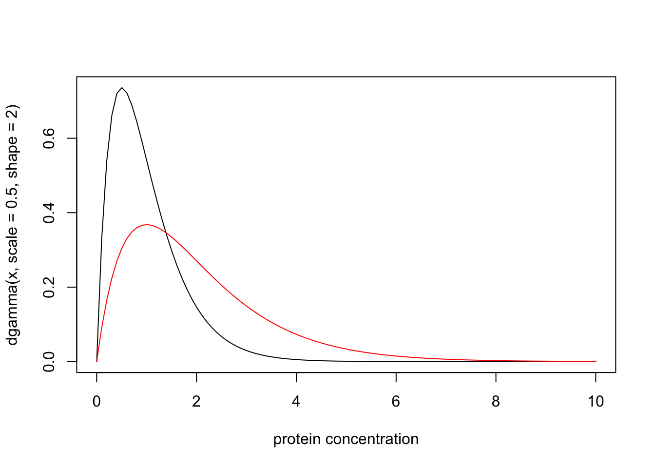
| Version | Author | Date |
|---|---|---|
| c3b365a | John Blischak | 2017-01-02 |
Suppose that for a particular patient we observe \(X=4.02\). Then the likelihood ratio for the model that this patient is from the normal group (\(M_n\)) vs the model that the patient is from the diseased group (\(M_d\)) is dgamma(4.02,scale=0.5,shape=2)/dgamma(4.02,scale=1,shape=2) which is 0.0718. That is, the data favour this individual being diseased by a factor of approximately 14.
Connection with Discrete Models
Often the likelihood ratio for continuous models is simply defined as the ratio of the densities, as above. However, an alternative approach, which can yield greater insight, is instead to derive this result as an approximation, from the definition of likelihood ratio for discrete models, as follows.
The first step is to recognize that in practice all observations are actually discrete, because of finite precision. Sometimes the measurement precision is made explicit, but often it is implicit in the number of decimal places used to report an observation. For example, in the example above, where we were told that we observed a protein concentration of \(X=4.02\), it would be reasonable to think that the measurement precision is 2 decimal places, and that this observation actually corresponds to “\(X\) lies in the interval \([4.015,4.025)\)”. The probability of this observation, under a continuous model for \(X\), is the integral of the probability density function from \(4.015\) to \(4.025\). In other words, it is\(F_X(4.025)-F_X(4.015)\) where \(F_X\) denotes the cumulative distribution function for \(X\).
With this view, the likelihood for the “observation” \(X=4.02\) under \(M_n\) is actually pgamma(4.025,scale=0.5,shape=2)-pgamma(4.015,scale=0.5,shape=2) = 5.1827928\times 10^{-5}. Similarly, the likelihood under \(M_d\) is 7.217107\times 10^{-4}, and the likelihood ratio is 0.0718126.
As you can see, this approach yields a LR that is numerically very close to that obtained using the ratio of the densities, as above. This is not a coincidence! Here is why we should expect this to happen more generally. Suppose we assume that measurement precision is \(\epsilon\). So the “observation” \(X=x\) really means \(X \in [x-\epsilon,x+\epsilon]\). Then the likelihood for a model \(M\), given this observation, is \(\Pr(X \in [x-\epsilon,x+\epsilon] | M)\). Provided that the density \(p(x|M)\) is approximately constant in the region within radius \(\epsilon\) around \(x\), then this probability is approximately \(2\epsilon p(x | M)\). Thus the LR for two models \(M_1\) vs \(M_0\), is given by
\[LR = \Pr(X \in [x-\epsilon,x+\epsilon] | M_1)/ \Pr(X \in [x-\epsilon,x+\epsilon] | M_0) \approx 2\epsilon p(x | M_1)/2\epsilon p(x|M_0) = p(x|M_1)/p(x|M_0).\]
An example where the approximation breaks down
The approximation usually works well, but here is a simple example to illustrate how the approximation could break down in principle.
Consider observing a single data point \(X\) and we compare the models that \(M_0: X \sim N(0,\sigma_0)\) vs \(M_1: X \sim N(0,\sigma_1)\). Suppose that we observe \(X=0.00\), assumed to be correct to the nearest 0.01. So the ``true" LR is given by
trueLR = function(s0,s1){
  L0= pnorm(0.005,sd=s0)-pnorm(-0.005,sd=s0)
  L1= pnorm(0.005,sd=s1)-pnorm(-0.005,sd=s1)
  return(L0/L1)
}
and the approximation is given by
approxLR = function(s0,s1){
  return(dnorm(0,sd=s0)/dnorm(0,sd=s1))
}
Now, if \(\sigma_0\) and \(\sigma_1\) are both not too small the the approximation works fine. For example, for \(\sigma_0,\sigma_1 = 0.5,1\) we have the truth and approximation as 1.999975 and 2.
But if one of the \(\sigma_j\) is small, we have the problem that the density is not approximately constant within the region \([-0.005,0.005]\). For example, at \(\sigma_0,\sigma_1 = 0.001,1\) we have the truth and approximation as 250.6637282 and 1000.
Summary
In most cases, the Likelihood ratio for model \(M_1\) vs model \(M_0\) for a continuous random variable \(X\), given an observation \(X=x\), can we well approximated by the ratio of the model densities of \(X\), evaluated at \(x\). This approximation comes from assuming that the model density functions are approximately constant within the neighborhood of \(x\) that has radius equal to the measurement precision.
sessionInfo()R version 3.5.2 (2018-12-20)
Platform: x86_64-apple-darwin15.6.0 (64-bit)
Running under: macOS Mojave 10.14.1
Matrix products: default
BLAS: /Library/Frameworks/R.framework/Versions/3.5/Resources/lib/libRblas.0.dylib
LAPACK: /Library/Frameworks/R.framework/Versions/3.5/Resources/lib/libRlapack.dylib
locale:
[1] en_US.UTF-8/en_US.UTF-8/en_US.UTF-8/C/en_US.UTF-8/en_US.UTF-8
attached base packages:
[1] stats graphics grDevices utils datasets methods base
loaded via a namespace (and not attached):
[1] workflowr_1.2.0 Rcpp_1.0.0 digest_0.6.18 rprojroot_1.3-2
[5] backports_1.1.3 git2r_0.24.0 magrittr_1.5 evaluate_0.12
[9] stringi_1.2.4 fs_1.2.6 whisker_0.3-2 rmarkdown_1.11
[13] tools_3.5.2 stringr_1.3.1 glue_1.3.0 xfun_0.4
[17] yaml_2.2.0 compiler_3.5.2 htmltools_0.3.6 knitr_1.21 This site was created with R Markdown