Conditional coverage of a frequentist CI
Matthew Stephens
2017-04-17
Last updated: 2019-03-31
Checks: 6 0
Knit directory: fiveMinuteStats/analysis/
This reproducible R Markdown analysis was created with workflowr (version 1.2.0). The Report tab describes the reproducibility checks that were applied when the results were created. The Past versions tab lists the development history.
Great! Since the R Markdown file has been committed to the Git repository, you know the exact version of the code that produced these results.
Great job! The global environment was empty. Objects defined in the global environment can affect the analysis in your R Markdown file in unknown ways. For reproduciblity it’s best to always run the code in an empty environment.
The command set.seed(12345) was run prior to running the code in the R Markdown file. Setting a seed ensures that any results that rely on randomness, e.g. subsampling or permutations, are reproducible.
Great job! Recording the operating system, R version, and package versions is critical for reproducibility.
Nice! There were no cached chunks for this analysis, so you can be confident that you successfully produced the results during this run.
Great! You are using Git for version control. Tracking code development and connecting the code version to the results is critical for reproducibility. The version displayed above was the version of the Git repository at the time these results were generated.
Note that you need to be careful to ensure that all relevant files for the analysis have been committed to Git prior to generating the results (you can use wflow_publish or wflow_git_commit). workflowr only checks the R Markdown file, but you know if there are other scripts or data files that it depends on. Below is the status of the Git repository when the results were generated:
Ignored files:
    Ignored:    .Rhistory
    Ignored:    .Rproj.user/
    Ignored:    analysis/.Rhistory
    Ignored:    analysis/bernoulli_poisson_process_cache/

Untracked files:
    Untracked:  _workflowr.yml
    Untracked:  analysis/CI.Rmd
    Untracked:  analysis/gibbs_structure.Rmd
    Untracked:  analysis/libs/
    Untracked:  analysis/results.Rmd
    Untracked:  analysis/shiny/tester/
    Untracked:  docs/MH_intro_files/
    Untracked:  docs/citations.bib
    Untracked:  docs/hmm_files/
    Untracked:  docs/libs/
    Untracked:  docs/shiny/tester/
Note that any generated files, e.g. HTML, png, CSS, etc., are not included in this status report because it is ok for generated content to have uncommitted changes.
These are the previous versions of the R Markdown and HTML files. If you’ve configured a remote Git repository (see ?wflow_git_remote), click on the hyperlinks in the table below to view them.
| File | Version | Author | Date | Message |
|---|---|---|---|---|
| html | 9905a6c | stephens999 | 2017-04-17 | Build site. |
| Rmd | 73bf57d | stephens999 | 2017-04-17 | Files commited by wflow_commit. |
Pre-requisite
You should be familiar with the result that if \(X \sim N(\theta,\sigma^2)\) then \(X \pm 1.96\sigma\) is a 95% Confidence Interval (CI) for \(\theta\).
Coverage vs Conditional Coverage
Suppose we consider going through life computing normal 95% CIs in lots of different situations.
That is, on occassion \(j\) (\(j=1,2,3,\dots\)) we observe data \[X_j | \theta_j, \sigma_j \sim N(\theta_j, \sigma_j),\] where \(\theta_j\) is unknown to us. For simplicity let us further assume that in each case the measurement error standard deviation, \(\sigma_j=1\), and is known to us.) Then we compute the standard 95% CI for \(\theta_j\): \[CI_j = [X_j -1.96, X_j + 1.96].\]
Consider now two questions:
What proportion of our intervals \(CI_j\) cover (contain) the true value of \(\theta_j\)?
Of the occasions when our interval \(CI_j\) excludes 0, what proportion will our interval cover the true value of \(\theta\)?
It is important to recognize that the answers to these two questions will be different.
The answer to i) is 95% because the definition of a 95% CI ensures this. This corresponds to the usual notion of the “coverage” of the CIs.
However, the answer to ii) will not generally be 95%. To see this, consider the extreme case where the \(\theta_j\) we consider over our life are all actually exactly equal to 0. Then the answer to the second question will be “never”!. More generally, the answer to ii) depends on the distribution of the actual \(\theta_j\) values that we consider during our life.
Illustration
Before setting out the analytic calculation, we will illustrate by simulation. Suppose first that the distribution of \(\theta_j\) we encounter over our life is \(N(0,s^2)\). Let us see by simulation how our answer to ii) depends on \(s\):
s = c(0.01,0.1,0.5,1,2,10,100)
nsim = 10000
coverage = rep(0,length(s))
cond_coverage = rep(0,length(s))
for(i in 1:length(s)){
  theta = rnorm(nsim, 0, s[i])
  X = rnorm(nsim, theta, 1)
  A = X-1.96
  B = X+1.96
  coverage[i] = mean(theta>A & theta< B)
  subset = (A>0 | B<0)
  cond_coverage[i] = mean(theta[subset]>A[subset] & theta[subset]<B[subset])
}
plot(log10(s),coverage,main="Coverage (black) and conditional coverage (red)", ylim=c(0,1), xlab="log_10(s)")
points(log10(s),cond_coverage,col="red")
abline(h=0.95,lty=2)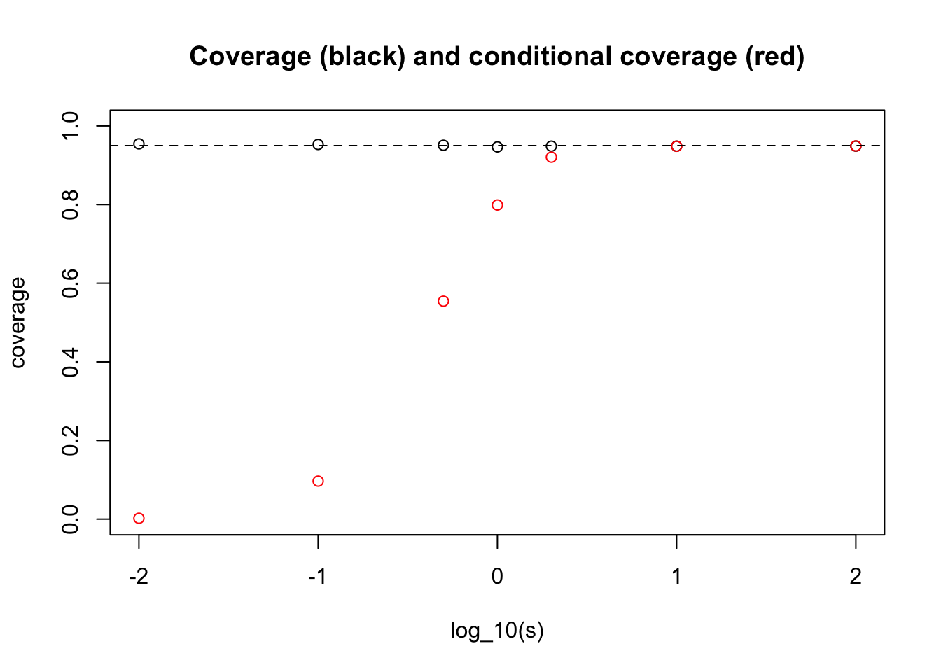
| Version | Author | Date |
|---|---|---|
| 9905a6c | stephens999 | 2017-04-17 |
What one can see here is that for very small \(s\) we get an answer close to the “never” answer that we discussed above (when \(\theta_j\) are identically 0).
And for large \(s\) we get the conditional coverage equal to 0.95. (This essentially follows from the result that in the limit \(s \rightarrow \infty\) the posterior distribution on \(\theta | X_j\) is \(N(X_j, 1)\).)
Analytic calculations
Actually computing the answer analytically here is not possible, but it is perhaps instructive to at least write out what we are (approximately) computing in the above simulation.
First, note that \(CI_j\) excludes 0 if and only if \(|X_j|>1.96\). So the probability we are asked to compute in ii) is \[\Pr( X_j - 1.96 < \theta_j < X_j + 1.96 | |X_j|>1.96).\] Computing this conditional distribution analytically leads to integrals of bivariate normal densities. The simulation above approximates this calculation (with error going to 0 as nsamp increases to infinity.)
sessionInfo()R version 3.5.2 (2018-12-20)
Platform: x86_64-apple-darwin15.6.0 (64-bit)
Running under: macOS Mojave 10.14.1
Matrix products: default
BLAS: /Library/Frameworks/R.framework/Versions/3.5/Resources/lib/libRblas.0.dylib
LAPACK: /Library/Frameworks/R.framework/Versions/3.5/Resources/lib/libRlapack.dylib
locale:
[1] en_US.UTF-8/en_US.UTF-8/en_US.UTF-8/C/en_US.UTF-8/en_US.UTF-8
attached base packages:
[1] stats graphics grDevices utils datasets methods base
loaded via a namespace (and not attached):
[1] workflowr_1.2.0 Rcpp_1.0.0 digest_0.6.18 rprojroot_1.3-2
[5] backports_1.1.3 git2r_0.24.0 magrittr_1.5 evaluate_0.12
[9] stringi_1.2.4 fs_1.2.6 whisker_0.3-2 rmarkdown_1.11
[13] tools_3.5.2 stringr_1.3.1 glue_1.3.0 xfun_0.4
[17] yaml_2.2.0 compiler_3.5.2 htmltools_0.3.6 knitr_1.21 This site was created with R Markdown