The Metropolis Hastings Algorithm
Matthew Stephens
April 23, 2018
Last updated: 2019-03-31
Checks: 6 0
Knit directory: fiveMinuteStats/analysis/
This reproducible R Markdown analysis was created with workflowr (version 1.2.0). The Report tab describes the reproducibility checks that were applied when the results were created. The Past versions tab lists the development history.
Great! Since the R Markdown file has been committed to the Git repository, you know the exact version of the code that produced these results.
Great job! The global environment was empty. Objects defined in the global environment can affect the analysis in your R Markdown file in unknown ways. For reproduciblity it’s best to always run the code in an empty environment.
The command set.seed(12345) was run prior to running the code in the R Markdown file. Setting a seed ensures that any results that rely on randomness, e.g. subsampling or permutations, are reproducible.
Great job! Recording the operating system, R version, and package versions is critical for reproducibility.
Nice! There were no cached chunks for this analysis, so you can be confident that you successfully produced the results during this run.
Great! You are using Git for version control. Tracking code development and connecting the code version to the results is critical for reproducibility. The version displayed above was the version of the Git repository at the time these results were generated.
Note that you need to be careful to ensure that all relevant files for the analysis have been committed to Git prior to generating the results (you can use wflow_publish or wflow_git_commit). workflowr only checks the R Markdown file, but you know if there are other scripts or data files that it depends on. Below is the status of the Git repository when the results were generated:
Ignored files:
    Ignored:    .Rhistory
    Ignored:    .Rproj.user/
    Ignored:    analysis/.Rhistory
    Ignored:    analysis/bernoulli_poisson_process_cache/

Untracked files:
    Untracked:  _workflowr.yml
    Untracked:  analysis/CI.Rmd
    Untracked:  analysis/gibbs_structure.Rmd
    Untracked:  analysis/libs/
    Untracked:  analysis/results.Rmd
    Untracked:  analysis/shiny/tester/
    Untracked:  docs/MH_intro_files/
    Untracked:  docs/citations.bib
    Untracked:  docs/hmm_files/
    Untracked:  docs/libs/
    Untracked:  docs/shiny/tester/
Note that any generated files, e.g. HTML, png, CSS, etc., are not included in this status report because it is ok for generated content to have uncommitted changes.
These are the previous versions of the R Markdown and HTML files. If you’ve configured a remote Git repository (see ?wflow_git_remote), click on the hyperlinks in the table below to view them.
| File | Version | Author | Date | Message |
|---|---|---|---|---|
| html | 6053d26 | stephens999 | 2018-04-23 | Build site. |
| Rmd | 1077c97 | stephens999 | 2018-04-23 | workflowr::wflow_publish(c(“analysis/index.Rmd”, “analysis/MH_intro.Rmd”, |
Prerequisites
You should be familiar with the concept of a Markov chain and its stationary distribution.
Introduction
The Metropolis Hastings algorithm is a beautifully simple algorithm for producing samples from distributions that may otherwise be difficult to sample from.
Suppose we want to sample from a distribution \(\pi\), which we will call the “target” distribution. For simplicity we assume that \(\pi\) is a one-dimensional distribution on the real line, although it is easy to extend to more than one dimension (see below).
The MH algorithm works by simulating a Markov Chain, whose stationary distribution is \(\pi\). This means that, in the long run, the samples from the Markov chain look like the samples from \(\pi\). As we will see, the algorithm is incredibly simple and flexible. Its main limitation is that, for difficult problems, “in the long run” may mean after a very long time. However, for simple problems the algorithm can work well.
The MH algorithm
The transition kernel
To implement the MH algorithm, the user (you!) must provide a “transition kernel”, \(Q\). A transition kernel is simply a way of moving, randomly, to a new position in space (\(y\) say), given a current position (\(x\) say). That is, \(Q\) is a distribution on \(y\) given \(x\), and we will write it \(Q(y | x)\). In many applications \(Q\) will be a continuous distribution, in which case \(Q(y|x)\) will be a density on \(y\), and so \(\int Q(y|x) dy =1\) (for all \(x\)).
For example, a very simple way to generate a new position \(y\) from a current position \(x\) is to add an \(N(0,1)\) random number to \(x\). That is, set \(y = x + N(0,1)\), or \(y|x \sim N(x,1)\). So \[Q(y | x) = 1/\sqrt{2\pi} \exp[-0.5(y-x)^2].\] This kind of kernel, which adds some random number to the current position \(x\) to obtain \(y\), is often used in practice and is called a “random walk” kernel.
Because of the role \(Q\) plays in the MH algorithm (see below), it is also sometimes called the “proposal distribution”. And the example given above would be called a “random walk proposal”.
The MH algorithm
The MH algorithm for sampling from a target distribution \(\pi\), using transition kernel \(Q\), consists of the following steps:
- Initialize, \(X_1 = x_1\) say.
For \(t=1,2,\dots\)
- sample \(y\) from \(Q(y | x_t)\). Think of \(y\) as a “proposed” value for \(x_{t+1}\).
- Compute \[A= \min \left( 1, \frac{\pi(y)Q(x_t | y)}{\pi(x_t)Q(y | x_t)} \right).\] \(A\) is often called the “acceptance probabilty”.
- with probability \(A\) “accept” the proposed value, and set \(x_{t+1}=y\). Otherwise set \(x_{t+1}=x_{t}\).
The Metropolis Algorithm
Notice that the example random walk proposal \(Q\) given above satisfies \(Q(y|x)=Q(x|y)\) for all \(x,y\). Any proposal that satisfies this is called “symmetric”. When \(Q\) is symmetric the formula for \(A\) in the MH algorithm simplifies to: \[A= \min \left( 1, \frac{\pi(y)}{\pi(x_t)} \right).\]
This special case of the algorithm, with \(Q\) symmetric, was first presented by Metropolis et al, 1953, and for this reason it is sometimes called the “Metropolis algorithm”.
In 1970 Hastings presented the more general version – now known as the MH algorithm – which allows that \(Q\) may be assymmetric. Specifically Hastings modified the acceptance probability by introducing the term \(Q(x_t|y)/Q(y|x_t)\). This ratio is sometimes called the “Hastings ratio”.
Toy Example
To help understand the MH algorithm we now do a simple example: we implement the algorithm to sample from an exponential distribution: \[\pi(x) = \exp(-x) \qquad (x \geq 0).\] Of course it would be much easier to sample from an exponential distribution in other ways; we are just using this to illustrate the algorithm.
Remember that \(\pi\) is called the “target” distribution, so we call our function to compute \(\pi\) target:
target = function(x){
  return(ifelse(x<0,0,exp(-x)))
}
Now we implement the MH algorithm, using the simple normal random walk transition kernel \(Q\) mentioned above. Since this \(Q\) is symmetric the Hastings ratio is 1, and we get the simpler form for the acceptance probability \(A\) in the Metropolis algorithm.
Here is the code:
x = rep(0,10000)
x[1] = 3     #initialize; I've set arbitrarily set this to 3
for(i in 2:10000){
  current_x = x[i-1]
  proposed_x = current_x + rnorm(1,mean=0,sd=1)
  A = target(proposed_x)/target(current_x)
  if(runif(1)<A){
    x[i] = proposed_x       # accept move with probabily min(1,A)
  } else {
    x[i] = current_x        # otherwise "reject" move, and stay where we are
  }
}
Having run this code we can plot the locations visited by the Markov chain \(x\) (sometimes called a trace plot).
plot(x,main="values of x visited by the MH algorithm")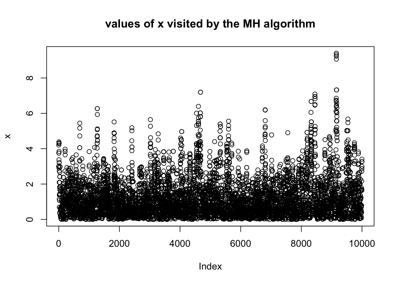
Remember that we designed this algorithm to sample from an exponential distribution. This means that (provided we ran the algorithm for long enough!) the histogram of \(x\) should look like an exponential distribution. Here we check this:
hist(x,xlim=c(0,10),probability = TRUE, main="Histogram of values of x visited by MH algorithm")
xx = seq(0,10,length=100)
lines(xx,target(xx),col="red")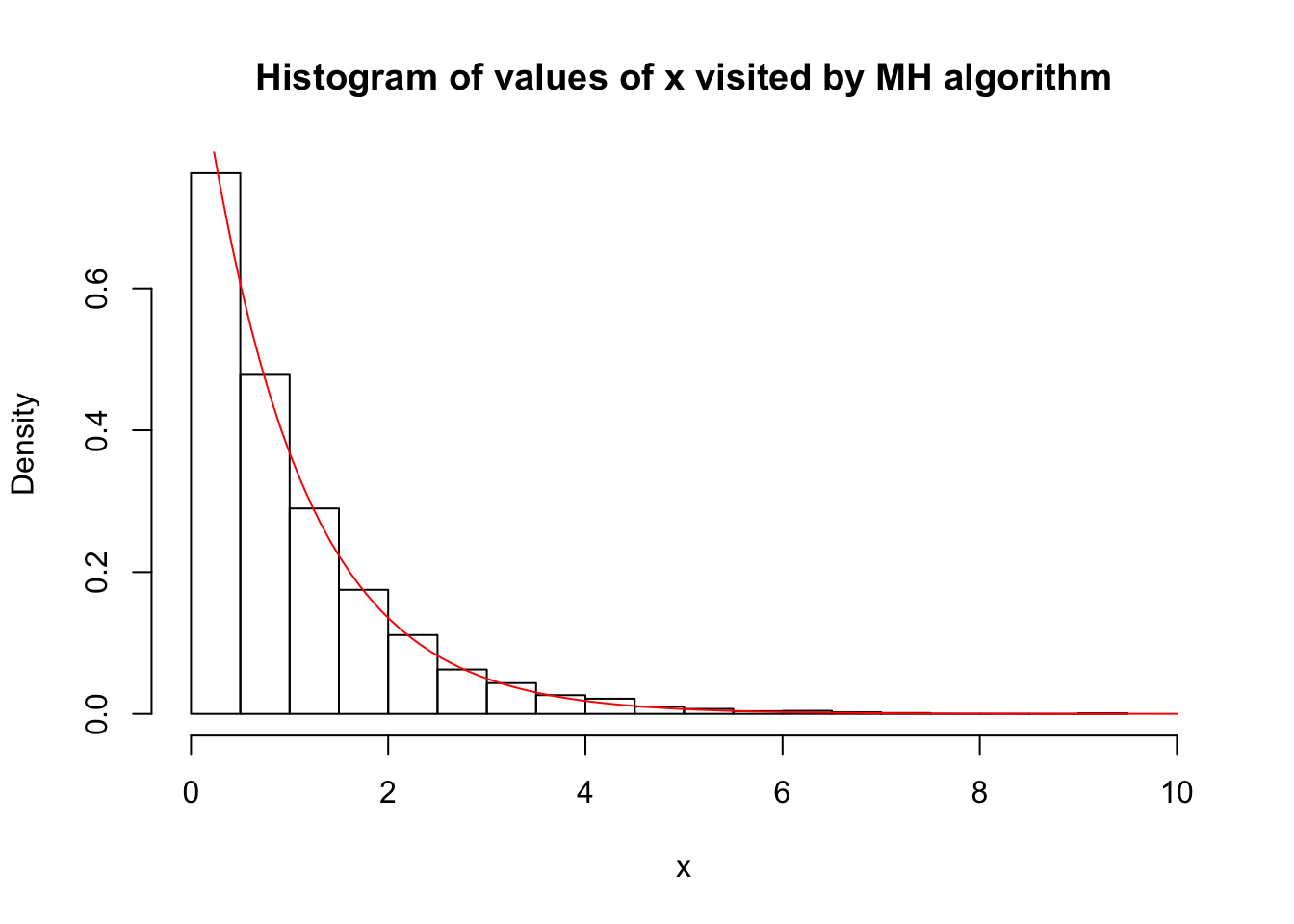 So we see that, indeed, the histogram of the values in \(x\) indeed provides a close fit to an exponential distribution.
Closing remarks
One particularly useful feature of the MH algorithm is that it can be implemented even when \(\pi\) is known only up to a constant: that is, \(\pi(x) = c f(x)\) for some known \(f\), but unknown constant \(c\). This is because the algorithm depends on \(\pi\) only through the ratio \(\pi(y)/\pi(x_t)=cf(y)/cf(x_t) = f(y)/f(x_t)\).
This issue arises in Bayesian applications, where the posterior distribution is proportional to the prior times the likelihood, but the constant of proportionality is often unknown. So the MH algorithm is particularly useful for sampling from posterior distributions to perform analytically-intractible Bayesian calculations.
sessionInfo()R version 3.5.2 (2018-12-20)
Platform: x86_64-apple-darwin15.6.0 (64-bit)
Running under: macOS Mojave 10.14.1
Matrix products: default
BLAS: /Library/Frameworks/R.framework/Versions/3.5/Resources/lib/libRblas.0.dylib
LAPACK: /Library/Frameworks/R.framework/Versions/3.5/Resources/lib/libRlapack.dylib
locale:
[1] en_US.UTF-8/en_US.UTF-8/en_US.UTF-8/C/en_US.UTF-8/en_US.UTF-8
attached base packages:
[1] stats graphics grDevices utils datasets methods base
loaded via a namespace (and not attached):
[1] workflowr_1.2.0 Rcpp_1.0.0 digest_0.6.18 rprojroot_1.3-2
[5] backports_1.1.3 git2r_0.24.0 magrittr_1.5 evaluate_0.12
[9] stringi_1.2.4 fs_1.2.6 whisker_0.3-2 rmarkdown_1.11
[13] tools_3.5.2 stringr_1.3.1 glue_1.3.0 xfun_0.4
[17] yaml_2.2.0 compiler_3.5.2 htmltools_0.3.6 knitr_1.21 This site was created with R Markdown