Likelihood Ratio: Wilks’s Theorem
Matt Bonakdarpour
2016-01-14
Last updated: 2019-03-31
Checks: 6 0
Knit directory: fiveMinuteStats/analysis/
This reproducible R Markdown analysis was created with workflowr (version 1.2.0). The Report tab describes the reproducibility checks that were applied when the results were created. The Past versions tab lists the development history.
Great! Since the R Markdown file has been committed to the Git repository, you know the exact version of the code that produced these results.
Great job! The global environment was empty. Objects defined in the global environment can affect the analysis in your R Markdown file in unknown ways. For reproduciblity it’s best to always run the code in an empty environment.
The command set.seed(12345) was run prior to running the code in the R Markdown file. Setting a seed ensures that any results that rely on randomness, e.g. subsampling or permutations, are reproducible.
Great job! Recording the operating system, R version, and package versions is critical for reproducibility.
Nice! There were no cached chunks for this analysis, so you can be confident that you successfully produced the results during this run.
Great! You are using Git for version control. Tracking code development and connecting the code version to the results is critical for reproducibility. The version displayed above was the version of the Git repository at the time these results were generated.
Note that you need to be careful to ensure that all relevant files for the analysis have been committed to Git prior to generating the results (you can use wflow_publish or wflow_git_commit). workflowr only checks the R Markdown file, but you know if there are other scripts or data files that it depends on. Below is the status of the Git repository when the results were generated:
Ignored files:
    Ignored:    .Rhistory
    Ignored:    .Rproj.user/
    Ignored:    analysis/.Rhistory
    Ignored:    analysis/bernoulli_poisson_process_cache/

Untracked files:
    Untracked:  _workflowr.yml
    Untracked:  analysis/CI.Rmd
    Untracked:  analysis/gibbs_structure.Rmd
    Untracked:  analysis/libs/
    Untracked:  analysis/results.Rmd
    Untracked:  analysis/shiny/tester/
    Untracked:  docs/MH_intro_files/
    Untracked:  docs/citations.bib
    Untracked:  docs/figure/MH_intro.Rmd/
    Untracked:  docs/figure/hmm.Rmd/
    Untracked:  docs/hmm_files/
    Untracked:  docs/libs/
    Untracked:  docs/shiny/tester/
Note that any generated files, e.g. HTML, png, CSS, etc., are not included in this status report because it is ok for generated content to have uncommitted changes.
These are the previous versions of the R Markdown and HTML files. If you’ve configured a remote Git repository (see ?wflow_git_remote), click on the hyperlinks in the table below to view them.
| File | Version | Author | Date | Message |
|---|---|---|---|---|
| html | 34bcc51 | John Blischak | 2017-03-06 | Build site. |
| Rmd | 5fbc8b5 | John Blischak | 2017-03-06 | Update workflowr project with wflow_update (version 0.4.0). |
| Rmd | 391ba3c | John Blischak | 2017-03-06 | Remove front and end matter of non-standard templates. |
| html | fb0f6e3 | stephens999 | 2017-03-03 | Merge pull request #33 from mdavy86/f/review |
| html | 0713277 | stephens999 | 2017-03-03 | Merge pull request #31 from mdavy86/f/review |
| Rmd | d674141 | Marcus Davy | 2017-02-27 | typos, refs |
| html | c3b365a | John Blischak | 2017-01-02 | Build site. |
| Rmd | 48e311e | John Blischak | 2017-01-02 | Simplify options for wilks.Rmd and remove intermediate md file. |
| Rmd | 67a8575 | John Blischak | 2017-01-02 | Use external chunk to set knitr chunk options. |
| Rmd | 5ec12c7 | John Blischak | 2017-01-02 | Use session-info chunk. |
| Rmd | 4fad37c | mbonakda | 2016-01-15 | fix URLs so they dont break if the page moves |
| Rmd | 3bcbe0d | mbonakda | 2016-01-14 | Merge branch ‘master’ into gh-pages |
| Rmd | 360c471 | mbonakda | 2016-01-14 | conform to template + ignore md files |
| Rmd | 8d87e30 | mbonakda | 2016-01-14 | fix wilks plots |
| Rmd | 3e7ba92 | mbonakda | 2016-01-14 | fix mathjax problem |
| Rmd | ff6b857 | mbonakda | 2016-01-12 | add asymptotic normality of MLE and wilks |
Pre-requisites
This document assumes familiarity with the concepts of likelihoods, likelihood ratios, and hypothesis testing.
Background
When performing a statistical hypothesis test, like comparing two models, if the hypotheses completely specify the probability distributions, these hypotheses are called simple hypotheses. For example, suppose we observe \(X_1,\ldots,X_n\) from a normal distribution with known variance and we want to test whether the true mean is equal to \(\mu_0\) or \(\mu_1\). One hypothesis \(H_0\) might be that the distribution has mean \(\mu_0\), and \(H_1\) might be that the mean is \(\mu_1\). Since these hypotheses completely specify the distribution of the \(X_i\), they are called simple hypotheses.
Now suppose \(H_0\) is again that the true mean, \(\mu\), is equal to \(\mu_0\), but \(H_1\) was that \(\mu > \mu_0\). In this case, the \(H_0\) is still simple, but \(H_1\) does not completely specify a single probability distribution. It specifies a set of distributions, and is therefore an example of a composite hypothesis. In most practical scenarios, both hypotheses are rarely simple.
As seen in the fiveMinuteStats on likelihood ratios, given the observed data \(X_1\ldots,X_n\), we can measure the relative plausibility of \(H_1\) to \(H_0\) by the log-likelihood ratio: \[\log\left(\frac{f(X_1,\ldots,X_n|H_1)}{f(X_1,\ldots,X_n|H_0)}\right)\]
The log-likelihood ratio could help us choose which model (\(H_0\) or \(H_1\)) is a more likely explanation for the data. One common question is this: what constitutes are large likelihood ratio? Wilks’s Theorem helps us answer this question – but first, we will define the notion of a generalized log-likelihood ratio.
Generalized Log-Likelihood Ratios
Let’s assume we are dealing with distributions parameterized by \(\theta\). To generalize the case of simple hypotheses, let’s assume that \(H_0\) specifies that \(\theta\) lives in some set \(\Theta_0\) and \(H_1\) specifies that \(\theta \in \Theta_1\). Let \(\Omega = \Theta_0 \cup \Theta_1\). A somewhat natural extension to the likelihood ratio test statistic we discussed above is the generalized log-likelihood ratio: \[\Lambda^* = \log{\frac{\max_{\theta \in \Theta_1}f(X_1,\ldots,X_n|\theta)}{\max_{\theta \in \Theta_0}f(X_1,\ldots,X_n|\theta)}}\]
For technical reasons, it is preferable to use the following related quantity:
\[\Lambda_n = 2\log{\frac{\max_{\theta \in \Omega}f(X_1,\ldots,X_n|\theta)}{\max_{\theta \in \Theta_0}f(X_1,\ldots,X_n|\theta)}}\]
Just like before, larger values of \(\Lambda_n\) provide stronger evidence against \(H_0\).
Wilks’s Theorem
Suppose that the dimension of \(\Omega = v\) and the dimension of \(\Theta_0 = r\). Under regularity conditions and assuming \(H_0\) is true, the distribution of \(\Lambda_n\) tends to a chi-squared distribution with degrees of freedom equal to \(v-r\) as the sample size tends to infinity.
With this theorem in hand (and for \(n\) large), we can compare the value of our log-likehood ratio to the expected values from a \(\chi^2_{v-r}\) distribution.
Example: Poisson Distribution
Assume we observe data \(X_1,\ldots X_n\) and consider the hypotheses \(H_0: \lambda = \lambda_0\) and \(H_1: \lambda \neq \lambda_0\). The likelihood is: \[L(\lambda|X_1,\ldots,X_n) = \frac{\lambda^{\sum X_i}e^{-n\lambda}}{\prod_i^n X_i!}\]
Note that \(\Theta_1\) in this case is the set of all \(\lambda \neq \lambda_0\). In the numerator of the expression for \(\Lambda_n\), we seek \(\max_{\theta \in \Omega}f(X_1,\ldots,X_n|\theta)\). This is just the maximum likelihood estimate of \(\lambda\) which we derived in this note. The MLE is simply the sample average \(\bar{X}\). The likelihood ratio is therefore: \[\frac{L(\lambda=\bar{X}|X_1,\ldots,X_n)}{L(\lambda=\lambda_0|X_1,\ldots,X_n)} = \frac{\bar{X}^{\sum X_i}e^{-n\bar{X}}}{\prod_i^n X_i!}\frac{\prod_i^n X_i!}{\lambda_0^{\sum X_i}e^{-n\lambda_0}} = \big ( \frac{\bar{X}}{\lambda_0}\big )^{\sum_i X_i}e^{n(\lambda_0 - \bar{X})}\]
which means that \(\Lambda_n\) is \[ \Lambda_n = 2\log{\left( \big ( \frac{\bar{X}}{\lambda_0}\big )^{\sum_i X_i}e^{n(\lambda_0 - \bar{X})} \right )} = 2n \left ( \bar{X}\log{\left(\frac{\bar{X}}{\lambda_0}\right)} + \lambda_0 - \bar{X} \right )\]
In this example we have that \(v\), the dimension of \(\Omega\), is 1 (any positive real number) and \(r\), the dimension of \(\Theta_0\) is 0 (it’s just a single point). Hence, the degrees of freedom of the asymptotic \(\chi^2\) distribution is \(v-r = 1\). Therefore, Wilk’s Theorem tells us that \(\Lambda_n\) tends to a \(\chi^2_1\) distribution as \(n\) tends to infinity.
Below we simulate computing \(\Lambda_n\) over 5000 experiments. In each experiment, we observe 500 random variables distributed as Poisson(\(0.4\)). We then plot the histogram of the \(\Lambda_n\)s and overlay the \(\chi^2_1\) density with a solid line.
num.iterations         <- 5000
lambda.truth           <- 0.4
num.samples.per.iter   <- 500
samples                <- numeric(num.iterations)
for(iter in seq_len(num.iterations)) {
  data            <- rpois(num.samples.per.iter, lambda.truth)
  samples[iter]   <- 2*num.samples.per.iter*(mean(data)*log(mean(data)/lambda.truth) + lambda.truth - mean(data))
}
hist(samples, freq=F, main='Histogram of LLR', xlab='sampled values of LLR values')
curve(dchisq(x, 1), 0, 20, lwd=2, xlab = "", ylab = "", add = T)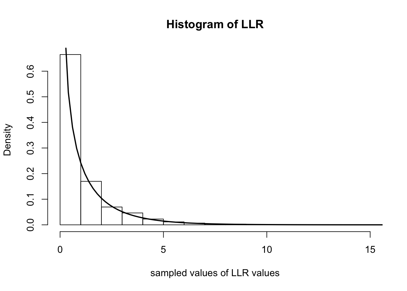
| Version | Author | Date |
|---|---|---|
| c3b365a | John Blischak | 2017-01-02 |
sessionInfo()R version 3.5.2 (2018-12-20)
Platform: x86_64-apple-darwin15.6.0 (64-bit)
Running under: macOS Mojave 10.14.1
Matrix products: default
BLAS: /Library/Frameworks/R.framework/Versions/3.5/Resources/lib/libRblas.0.dylib
LAPACK: /Library/Frameworks/R.framework/Versions/3.5/Resources/lib/libRlapack.dylib
locale:
[1] en_US.UTF-8/en_US.UTF-8/en_US.UTF-8/C/en_US.UTF-8/en_US.UTF-8
attached base packages:
[1] stats graphics grDevices utils datasets methods base
loaded via a namespace (and not attached):
[1] workflowr_1.2.0 Rcpp_1.0.0 digest_0.6.18 rprojroot_1.3-2
[5] backports_1.1.3 git2r_0.24.0 magrittr_1.5 evaluate_0.12
[9] stringi_1.2.4 fs_1.2.6 whisker_0.3-2 rmarkdown_1.11
[13] tools_3.5.2 stringr_1.3.1 glue_1.3.0 xfun_0.4
[17] yaml_2.2.0 compiler_3.5.2 htmltools_0.3.6 knitr_1.21 This site was created with R Markdown