The Beta Distribution
Matthew Stephens
2017-01-25
Last updated: 2017-03-06
Code version: c7339fc
Overview
The purpose of this vignette is to introduce the Beta distribution. You should be familiar with basic concepts related to distributions before - e.g. maybe you have come across the normal distribution and a uniform distribution before, and understand what it would mean to talk about their mean, variance and density.
If you want more details you could look at Wikipedia.
The Beta Distribution
The Beta distribution is a distribution on the interval \([0,1]\). Probably you have come across the \(U[0,1]\) distribution before: the uniform distribution on \([0,1]\). You can think of the Beta distribution as a generalization of this that allows for some simple non-uniform distributions for values between 0 and 1.
The Beta distribution has two parameters, which we will call \(a\) and \(b\). These two parameters determine the shape of the Beta distributions (just as the mean and variance determine the shape of the normal distribution).
Following the usual convention, we will write \(X \sim Be(a,b)\) as shorthand for “\(X\) has a Beta distribution with parameters \(a\) and \(b\)”.
Density
If \(X \sim Be(a,b)\) then the density of \(X\) is: \[f_X(x) = \frac{1}{B(a,b)} x^{a-1}(1-x)^{b-1} \qquad (x \in [0,1]).\]
For those of you that are interested, \(B(a,b)\) is known as the “beta function” and is given by the integral \[B(a,b) = \int_0^1 x^{a-1} (1-x)^{b-1} \,dx.\] This is where the beta distribution gets its name: its density involves the beta function. However, for this introduction you do not have to worry very much about what \(B(a,b)\) is: think of it as a constant (in that it does not depend on \(x\)), that is included so that the density integrates to 1, as all densities must.
Because the Beta distribution is widely used, R has the built in function dbeta to compute this density. We will use this to look at some examples of the Beta distribution below.
Examples
First we will look at some examples for \(a=b\), with both \(\geq 1\):
p = seq(0,1, length=100)
plot(p, dbeta(p, 100, 100), ylab="density", type ="l", col=4)
lines(p, dbeta(p, 10, 10), type ="l", col=3)
lines(p, dbeta(p, 2, 2), col=2)
lines(p, dbeta(p, 1, 1), col=1)
legend(0.7,8, c("Be(100,100)","Be(10,10)","Be(2,2)", "Be(1,1)"),lty=c(1,1,1,1),col=c(4,3,2,1))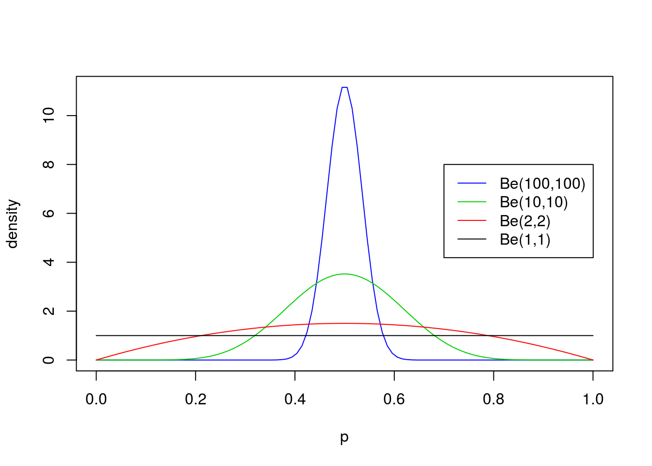
Now non-equal values of \(a\) and \(b\) with both \(\geq 1\):
p = seq(0,1, length=100)
plot(p, dbeta(p, 900, 100), ylab="density", type ="l", col=4)
lines(p, dbeta(p, 90, 10), type ="l", col=3)
lines(p, dbeta(p, 30, 70), col=2)
lines(p, dbeta(p, 3, 7), col=1)
legend(0.2,30, c("Be(900,100)","Be(90,10)","Be(30,70)", "Be(3,7)"),lty=c(1,1,1,1),col=c(4,3,2,1))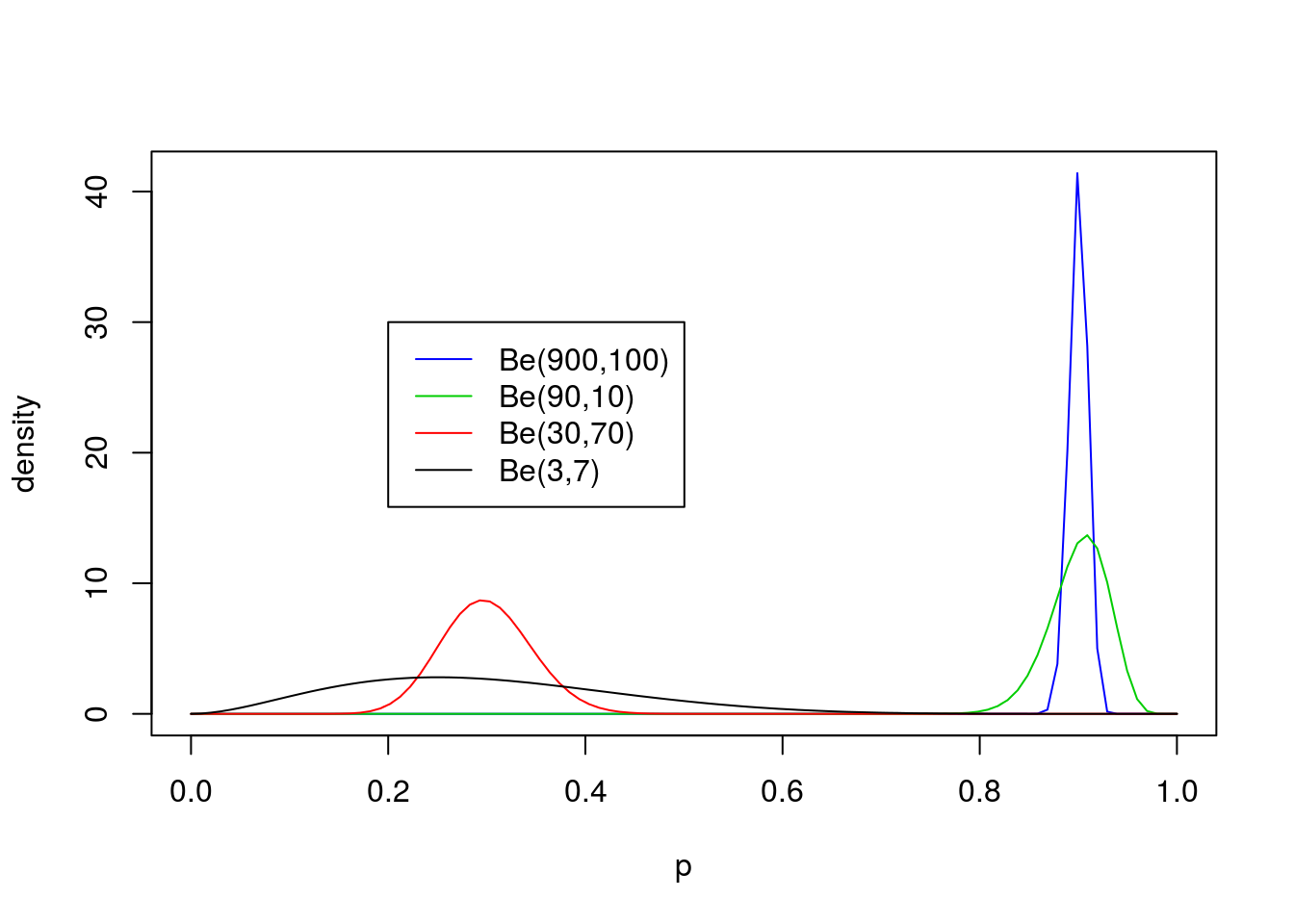
From these examples you should note the following:
- The distribution is roughly centered on \(a/(a+b)\). Actually, it turns out that the mean is exactly \(a/(a+b)\). Thus the mean of the distribution is determined by the relative values of \(a\) and \(b\).
- The larger the values of \(a\) and \(b\), the smaller the variance of the distribution about the mean.
- For moderately large values of \(a\) and \(b\) the distribution looks visually “kind of normal”, although unlike the normal distribution the Beta distribution is restricted to [0,1].
- The special case \(a=b=1\) is the uniform distribution.
Values of \(a,b <1\)
The parameters \(a\) and \(b\) can also be less than 1, but the distribution in this case starts to have a different kind of shape. Specifically if \(a<1\) then there is a peak at 0, and if \(b<1\) then there is a peak at 1 (so if both are \(<1\) then the distribution is U-shaped). Here are some examples:
p = seq(0,1, length=100)
plot(p, dbeta(p, 0.1, 0.1), ylab="density", type ="l", col=4)
lines(p, dbeta(p, 0.5, 0.5), type ="l", col=3)
lines(p, dbeta(p, 0.1, 0.5), col=2)
lines(p, dbeta(p, 0.5, 2), col=1)
legend(0.5,2, c("Be(0.1,0.1)","Be(0.5,0.5)","Be(0.1,0.5)", "Be(0.5,2)"),lty=c(1,1,1,1),col=c(4,3,2,1))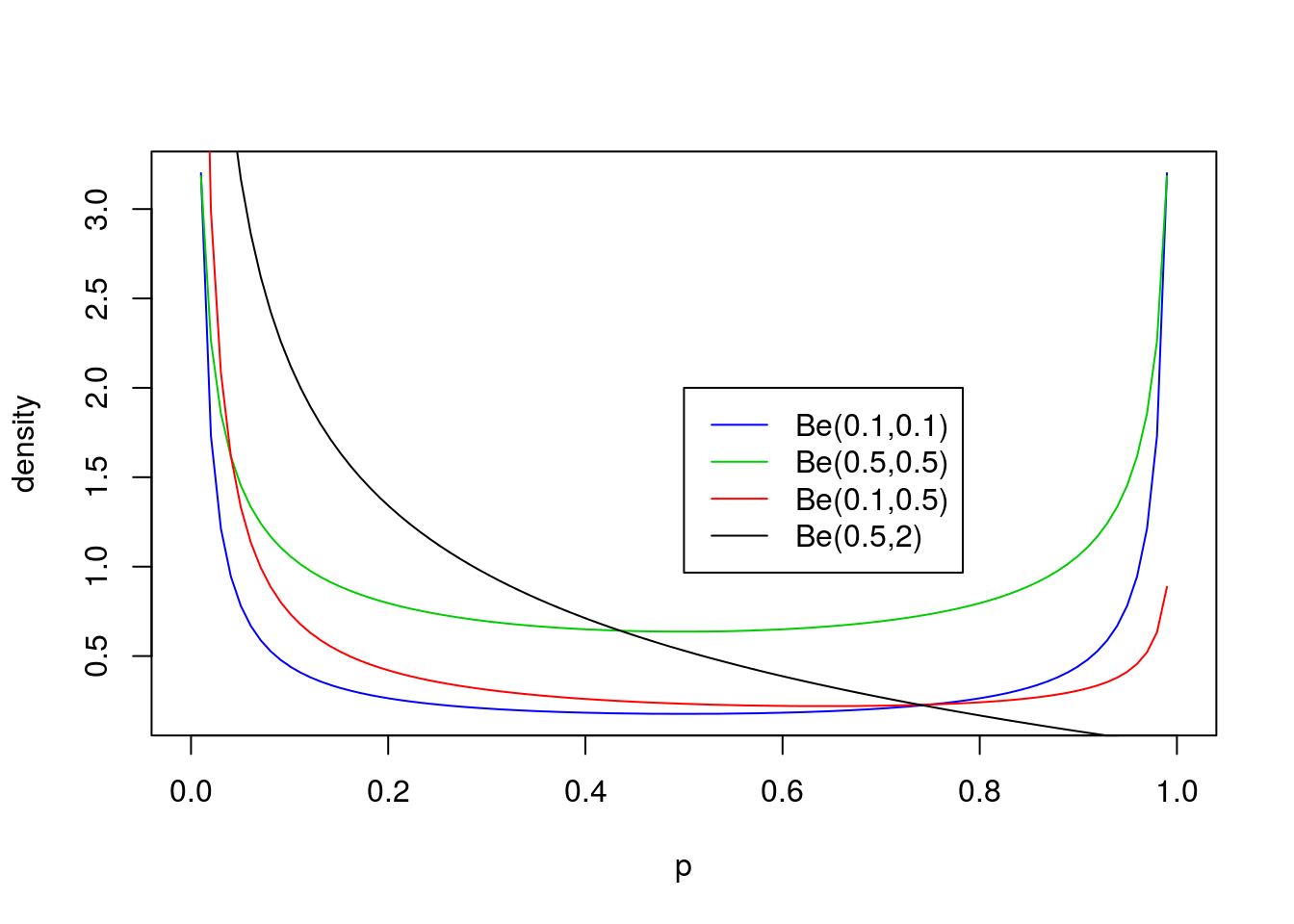
Exercise
- Sketch what you think the Be(5,5) and Be(0.5,5) and Be(500,200) distributions would look like. Check your sketches against the truth computed using
dbeta.
Session information
sessionInfo()R version 3.3.2 (2016-10-31)
Platform: x86_64-pc-linux-gnu (64-bit)
Running under: Ubuntu 14.04.5 LTS
locale:
[1] LC_CTYPE=en_US.UTF-8 LC_NUMERIC=C
[3] LC_TIME=en_US.UTF-8 LC_COLLATE=en_US.UTF-8
[5] LC_MONETARY=en_US.UTF-8 LC_MESSAGES=en_US.UTF-8
[7] LC_PAPER=en_US.UTF-8 LC_NAME=C
[9] LC_ADDRESS=C LC_TELEPHONE=C
[11] LC_MEASUREMENT=en_US.UTF-8 LC_IDENTIFICATION=C
attached base packages:
[1] stats graphics grDevices utils datasets methods base
other attached packages:
[1] workflowr_0.4.0 rmarkdown_1.3.9004
loaded via a namespace (and not attached):
[1] backports_1.0.5 magrittr_1.5 rprojroot_1.2 htmltools_0.3.5
[5] tools_3.3.2 yaml_2.1.14 Rcpp_0.12.9 stringi_1.1.2
[9] knitr_1.15.1 git2r_0.18.0 stringr_1.2.0 digest_0.6.12
[13] evaluate_0.10 This site was created with R Markdown